Article Catalog
- Blogger’s Boutique Column Navigation
- Note: The following source code can be run, different projects involved in the function are analyzed in detail.
- 11、Image project practice
- (i) Bank card number identification — sort_contours(), resize()
- (ii) document scanning OCR recognition — cv2.getPerspectiveTransform() + cv2.warpPerspective(), np.argmin(), np.argmax(), np.diff()
- detectAndDescribe(), matchKeypoints(), cv2.findHomography(), cv2.warpPerspective(), drawMatches()
- (iv) Parking lot space detection (Keras-based CNN classification) — pickle.dump(), pickle.load(), cv2.fillPoly(), cv2.bitwise_and(), cv2.circle(), cv2. HoughLinesP(), cv2.line()
- (v) Answer key recognition and marking — cv2.putText(), cv2.countNonZero()
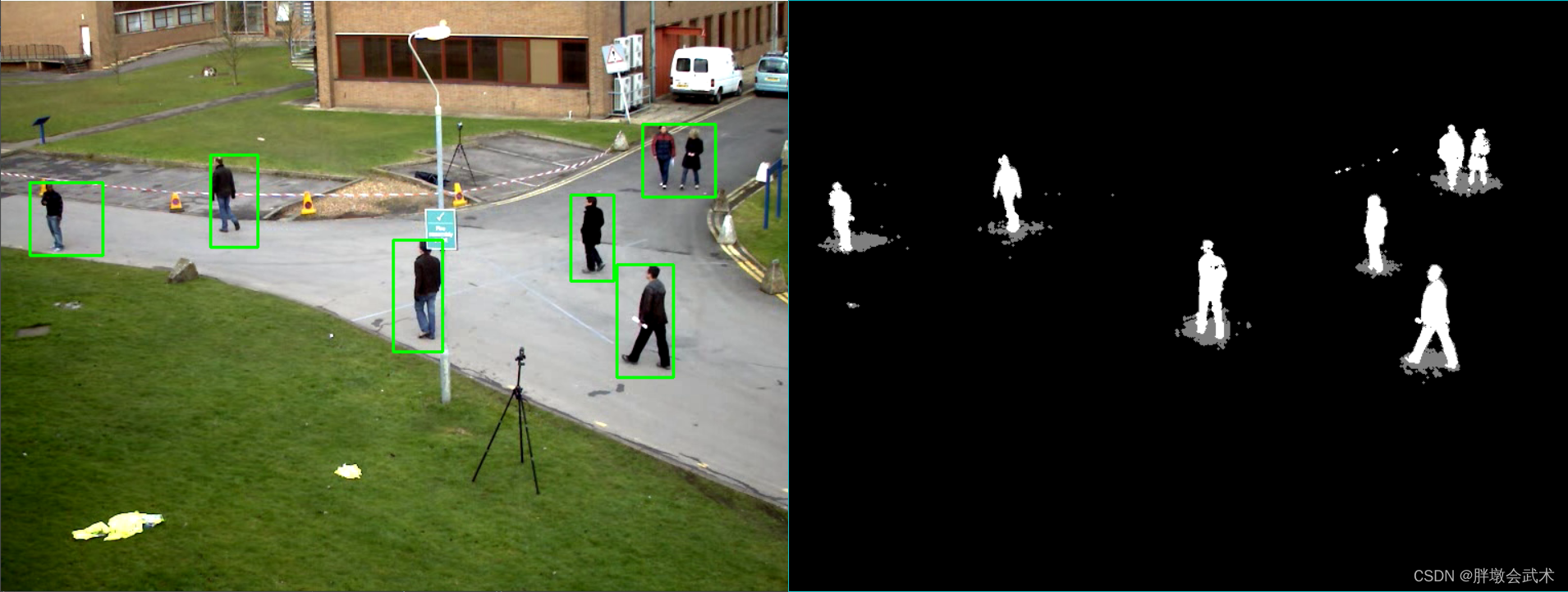
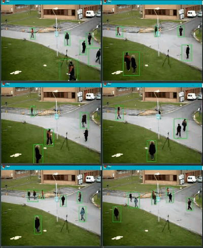
- (vi) Background modeling (dynamic target recognition) — cv2.getStructuringElement(), cv2.createBackgroundSubtractorMOG2()
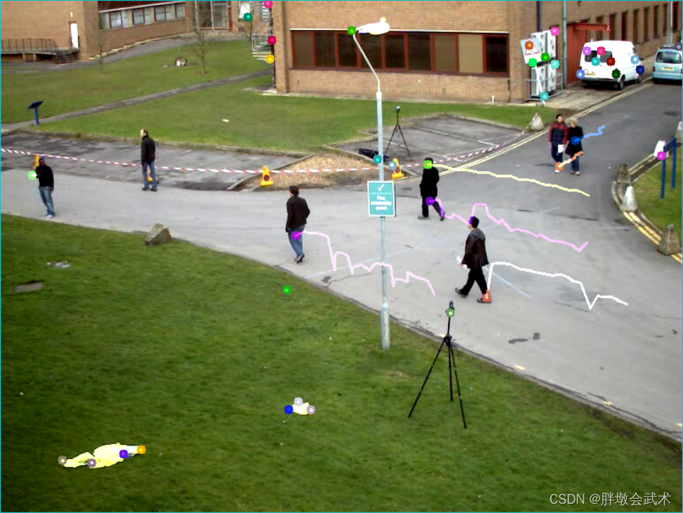
- (vii) Optical flow estimation (track point tracking) – cv2.goodFeaturesToTrack(), cv2.calcOpticalFlowPyrLK()
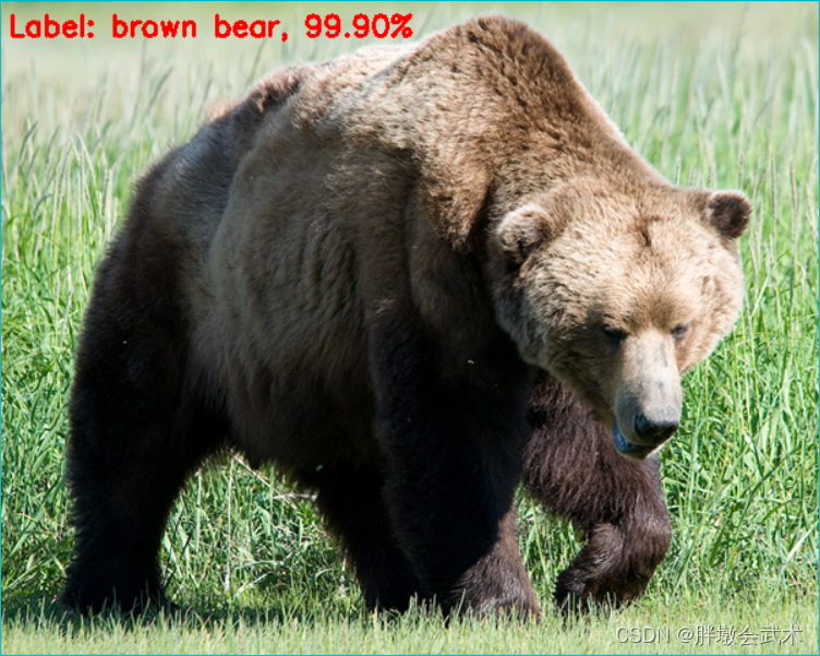
- (viii) Classification of DNN modules — cv2.dnn.blobFromImage()
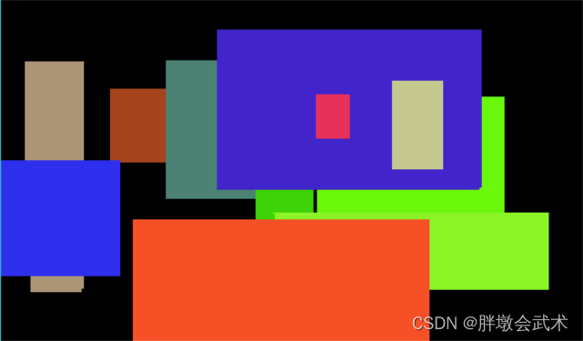
- (ix) Rectangular Doodle Drawing Board — cv.namedWindow(), cv.setMouseCallback()
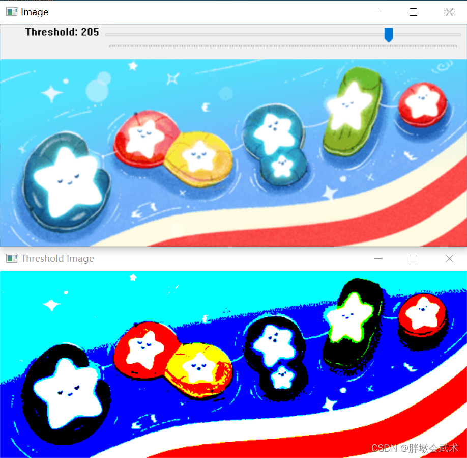
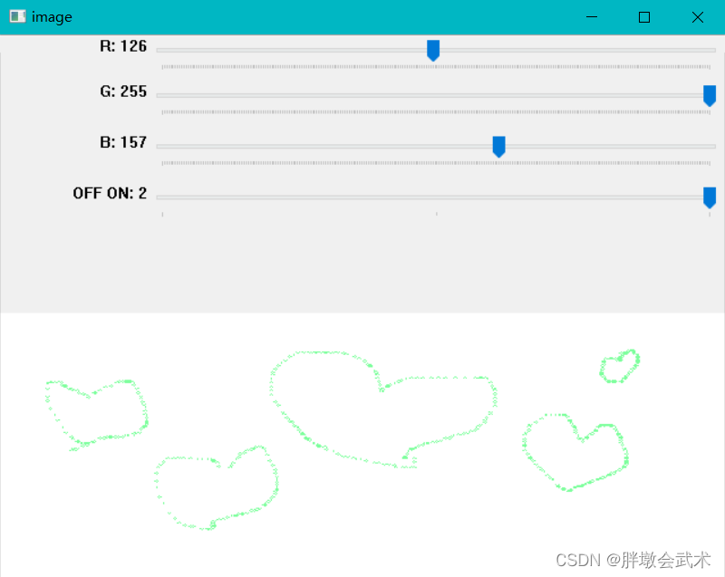
- (x) create trackbar — createTrackbar(), cv2.getTrackbarPos()
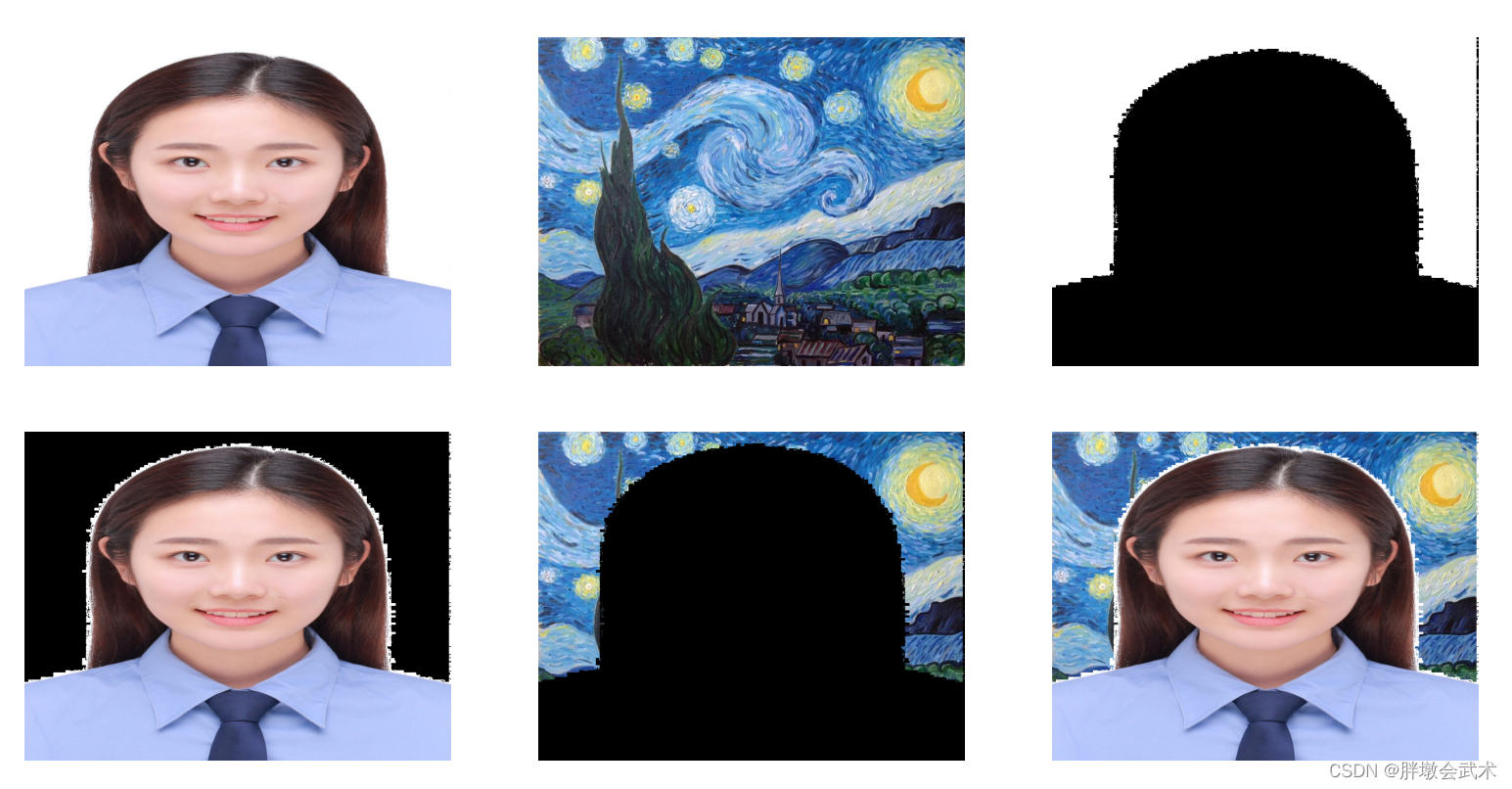
- (xi) binary-based implementation of portrait keying and background replacement — np.where(), np.uint8()
- 22. Basic image operation
- (i) Image reading, saving and displaying — cv2.imread(), cv2.imwrite(), cv2.imshow()
- (ii) Video reading and processing — cv2.VideoCapture()
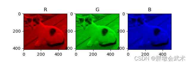
- (iii) Tricolor map of the image — cv2.split() + cv.merge()
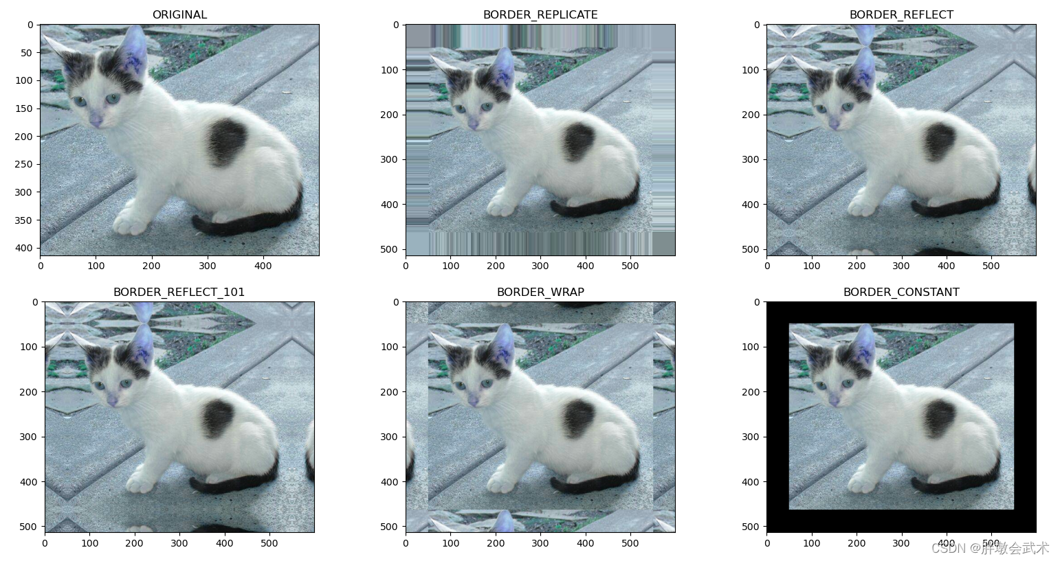
- (iv) Edge filling of an image — cv2.copyMakeBorder()
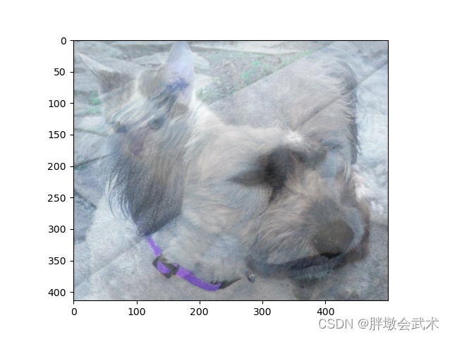
- (v) image fusion — cv2.addWeighted()
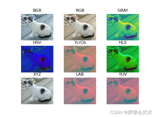
- (vi) color space conversion — cv2.cvtColor()
- (vii) Thresholding — cv2.threshold() + cv2.adaptiveThreshold()
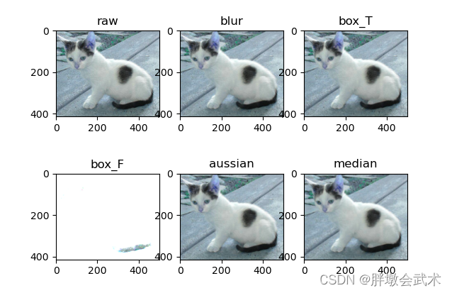
- (viii) Mean/Gaussian/box/median filter — cv2.blur() + cv2.boxFilter() + cv2.GaussianBlur() + cv2.medianBlur()
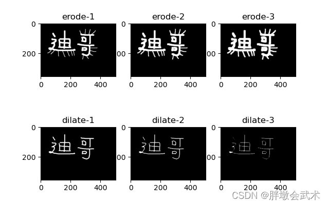
- (ix) Erosion and dilation — cv2.erode() vs. cv2.dilate() + np.zeros() vs. np.ones()
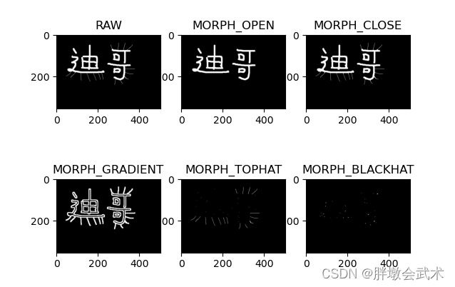
- (x) Morphological changes — cv2.morphologyEx()
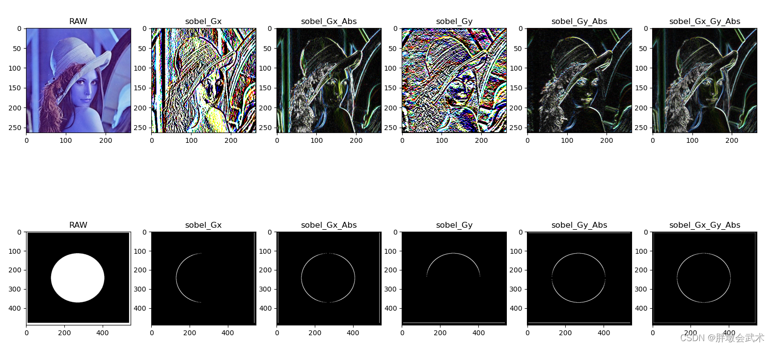
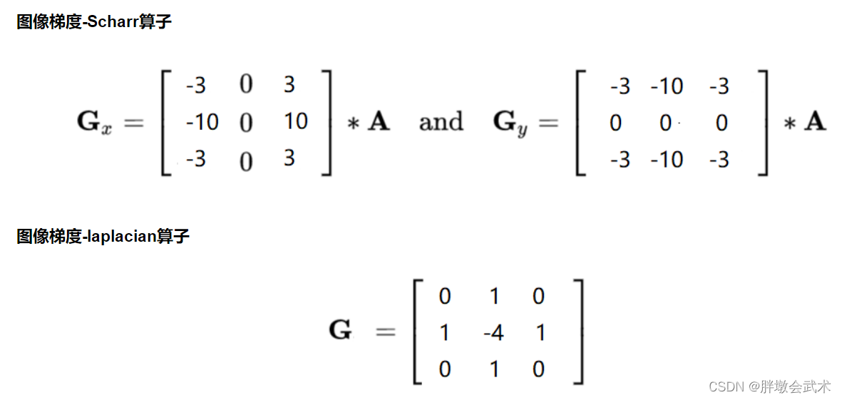
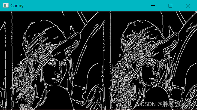
- (xi) Edge detection operators — cv2.sobel(), cv2.Scharr(), cv2.Laplacian(), cv2.Canny()
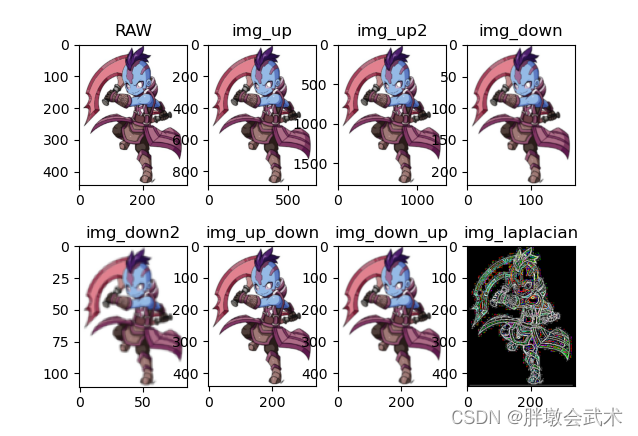
- (xii) Image pyramid — cv2.pyrUp(), cv2.pyrDown()
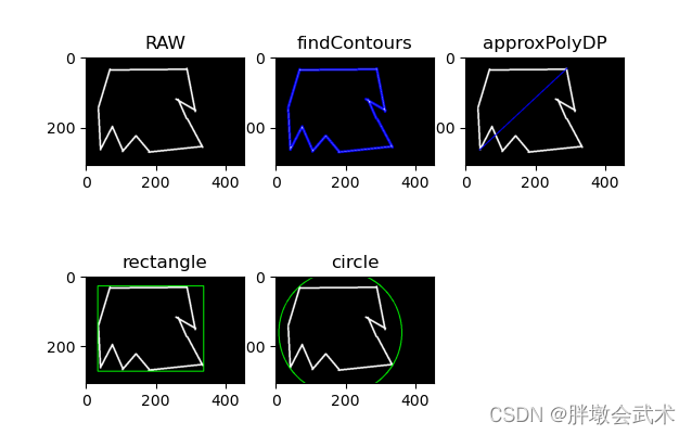
- (xiii) image contour detection — cv2.findContours(), cv2.drawContours(), cv2.arcLength(), cv2.approxPolyDP(), cv2.rectangle()
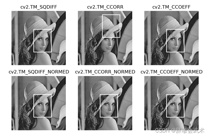
- (xiv) template matching — cv2.matchTemplate(), cv2.minMaxLoc()
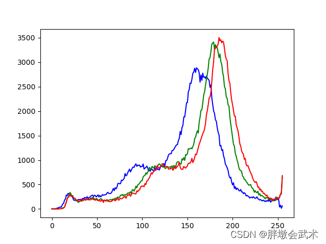
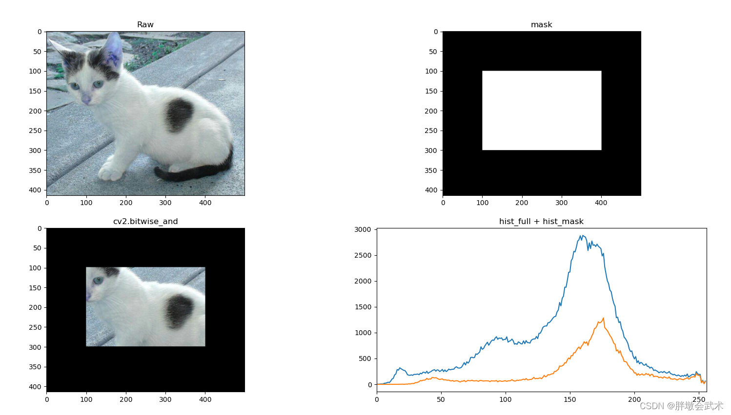
- (xv) Histogram (equalize) — cv2.calcHist(), img.ravel(), cv2.bitwise_and(), cv2.equalizeHist(), cv2.createCLAHE()
- (xvi) Fourier transform + lowpass/highpass filtering — cv2.dft(), cv2.idft(), np.fft.fftshift(), np.fft.ifftshift(), cv2.magnitud()
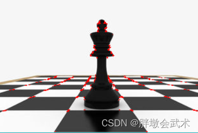
- (xvii) Harris corner detection — cv2.cornerHarris(), np.float32()
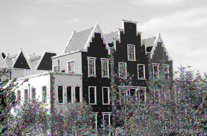
- (xviii) SIFT scale-invariant feature detection — cv2.xfeatures2d.SIFT_create(), sift.detectAndCompute(), sift.detect(), sift.compute(), cv2. drawKeypoints
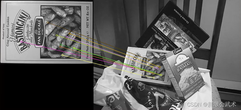
- (xix) Violent feature matching — cv2.BFMatcher_create(), bf.match(), bf_knn.knnMatch(), cv2.drawMatches()
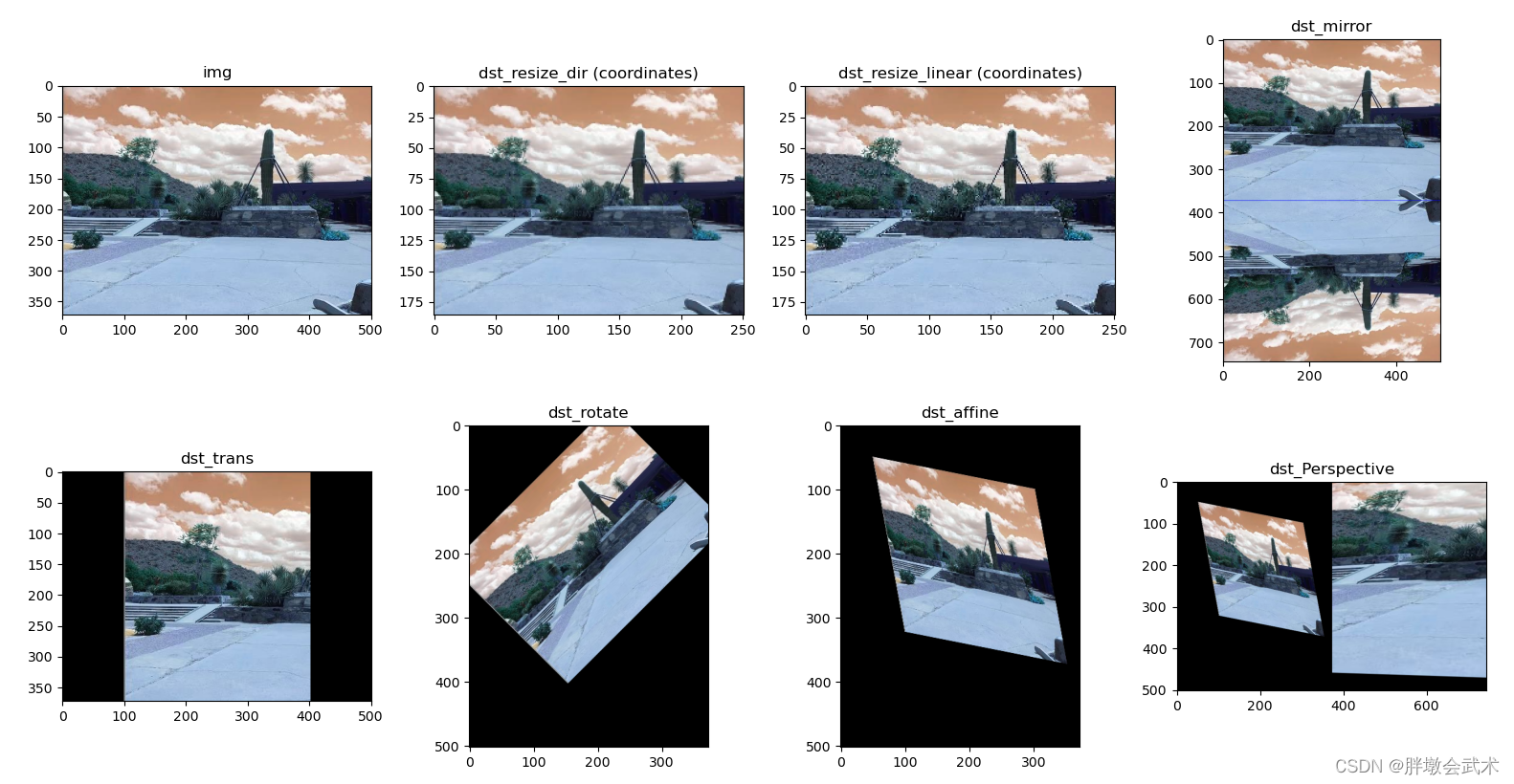
- (xx) Image scaling + mirroring + translation + rotation + affine transformation + perspective transformation — cv2.resize(), cv2.getRotationMatrix2D(), cv2.getAffineTransform(), cv2. getPerspectiveTransform(), cv2.warpPerspective(), cv2.warpAffine()
Blogger’s Boutique Column Navigation
- 🍕 Column:Pytorch project in practice
- 🌭 Opencv Image Processing (full)
- 🍱 Opencv C++ Image Processing (full)
- 🍳 Pillow Image Processing (PIL.Image)
- 🍝 Pytorch Basics (full)
- 🥙 Python common built-in functions (all)
- 🍰 Classical models of convolutional neural networks CNN
- 🍟 Hands-on knowledge of Convolutional Neural Networks CNNs
- 🥘 Thirty thousand words of hardcore detail: yolov1, yolov2, yolov3, yolov4, yolov5, yolov7
Note: The following source code can be run, different projects involved in the function are analyzed in detail.
11、Image project practice
(i) Bank card number identification — sort_contours(), resize()
[Credit card testing process explained in detail]
11. Extract each number of the template
1111, read template image, convert to grayscale map, convert to binary map
1122, contour detection, drawing of contours, sorting of all contours obtained (numbering)
1133, Extract all contours of the template – every number
22. Extract all the outlines of the credit card
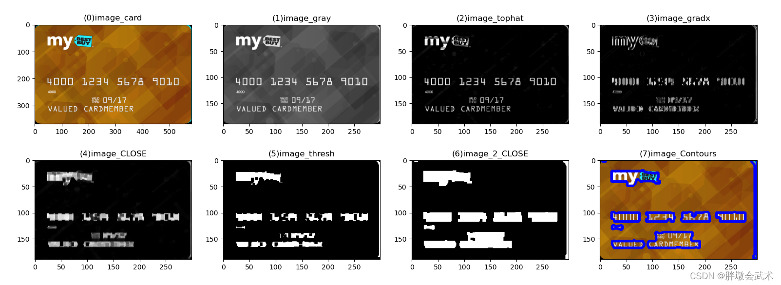
2211, read image to be detected, convert to grayscale, top hat operation, sobel operator operation, closure operation, binarization, quadratic expansion + erosion
2222, Contour detection, Contour drawing
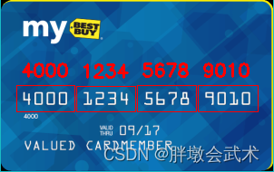
33, extract the bank card “a group of four numbers” outline, and then each outline with the template of each number to match, get the maximum matching results
3311. Among all the contours, identify the contours of A Set of Four Numbers (there are four in total), and perform thresholding, contour detection, and contour ranking
3322, In A Set of Four Numbers, extract the outline as well as the coordinates of each number and perform template matching to get the maximum matching result
44. On the original image, use a rectangle to draw a “group of four numbers” and display all the matching results on the original image
import cv2 # opencv reads in BGR format
import matplotlib.pyplot as plt # Matplotlib is RGB
import numpy as np
def sort_contours(cnt_s, method="left-to-right"):
reverse = False
ii_myutils = 0
if method == "right-to-left" or method == "bottom-to-top":
reverse = True
if method == "top-to-bottom" or method == "bottom-to-top":
ii_myutils = 1
bounding_boxes = [cv2.boundingRect(cc_myutils) for cc_myutils in cnt_s] # Wrap the found shapes with a minimal rectangle x,y,h,w
(cnt_s, bounding_boxes) = zip(*sorted(zip(cnt_s, bounding_boxes), key=lambda b: b[1][ii_myutils], reverse=reverse))
return cnt_s, bounding_boxes
def resize(image, width=None, height=None, inter=cv2.INTER_AREA):
dim_myutils = None
(h_myutils, w_myutils) = image.shape[:2]
if width is None and height is None:
return image
if width is None:
r_myutils = height / float(h_myutils)
dim_myutils = (int(w_myutils * r_myutils), height)
else:
r_myutils = width / float(w_myutils)
dim_myutils = (width, int(h_myutils * r_myutils))
resized = cv2.resize(image, dim_myutils, interpolation=inter)
return resized
######################################################################
# 11. Extract each number of the template
######################################################################
# Read template images (bank cards correspond to number templates from 0 to 9)
img = cv2.imread(r'ocr_a_reference.png')
ref_gray = cv2.cvtColor(img, cv2.COLOR_BGR2GRAY) # convert to grayscale
ref_BINARY = cv2.threshold(ref_gray, 10, 255, cv2.THRESH_BINARY_INV)[1] # Convert to binary image
"""#######################################
contours, hierarchy = cv2.findContours(img, mode, method)
# Input parameter mode: contour retrieval mode
# (1) RETR_EXTERNAL: Retrieves only the outermost contour;
# (2) RETR_LIST: Retrieves all contours, but the detected contours are not hierarchically related and are stored in a linked list.
# (3) RETR_CCOMP: Retrieves all contours and creates two levels of contours. The top level is the outer boundaries of the parts and the inner level is the boundary information; the
# (4) RETR_TREE: Retrieves all profiles and builds a hierarchical tree structure of profiles; (most commonly used)
# method: contour approximation method
# (1) CHAIN_APPROX_NONE: Stores all contour points where the pixel position difference between two neighboring points is no more than 1. Example: four edges of a matrix. (most commonly used)
# (2) CHAIN_APPROX_SIMPLE: Compresses elements in the horizontal, vertical, and diagonal directions, keeping only the endpoint coordinates in that direction.   Example: 4 contour points of a rectangle.
# Output parameters contours: all contours
# hierarchy: attributes corresponding to each profile
# Note 0: A contour is a curve that joins consecutive points (with boundaries) together, with the same color or gray scale. Contours are useful in shape analysis and object detection and recognition.
# Note 1: The function input image is a binary map, i.e. black and white (not grayscale). So the read image should be converted to grayscale first, and then to binary map.
# Note 2: The function returns only two values in opencv2: contours, hierarchy.
# Note 3: The function returns three values in opencv3: img, countours, hierarchy
#######################################"""
refCnts, hierarchy = cv2.findContours(ref_BINARY.copy(), cv2.RETR_EXTERNAL, cv2.CHAIN_APPROX_SIMPLE)
"""#######################################
# draw contours: v2.drawContours(image, contours, contourIdx, color, thickness) ---- (on image) draws the contours of the image
# Input parameter image: target image to draw the outline on, note that it will change the original image.
# contours: contour points, the first return value of the above cv2.findContours() function
# contourIdx: index of the contour, indicates the first contour to be drawn. -1 means all contours are drawn
# color: the color (RGB) to draw the outline in
# thickness: (optional parameter) the width of the contour line, -1 for fill
# Note: The image needs a copy of copy() first, otherwise (the image of the assignment operation) and the original image will change together.
#######################################"""
img_Contours = img.copy()
cv2.drawContours(img_Contours, refCnts, -1, (0, 0, 255), 3)
# print(np.array(refCnts).shape)
# Drawing (image processing and obtaining graphical display of contours)
plt.subplot(221), 	plt.imshow(img, 'gray'),            plt.title('(0)ref')
plt.subplot(222), 	plt.imshow(ref_gray, 'gray'),       plt.title('(1)ref_gray')
plt.subplot(223), 	plt.imshow(ref_BINARY, 'gray'),     plt.title('(2)ref_BINARY')
plt.subplot(224), 	plt.imshow(img_Contours, 'gray'),   plt.title('(3)img_Contours')
plt.show()
#######################################
# Sort (number) all resulting contours: left to right, top to bottom
refCnts = sort_contours(refCnts, method="left-to-right")[0]
#######################################
# Extract all the contours (of the template) - Numeric
digits = {} # hold the digits of each template - tuple initialization
for (i, c) in enumerate(refCnts):
(x, y, w, h) = cv2.boundingRect(c) # get the (x, y) coordinates, width and length of the upper left corner of the outer rectangle of the outline (number)
roi = ref_BINARY[y:y + h, x:x + w] # get the coordinates of the outer rectangle
roi = cv2.resize(roi, (57, 88)) # resize the image of the region of interest (numbers) to the same size
digits[i] = roi # save each template (digit)
######################################################################
# 22. Extract all the outlines of the credit card
"""######################################################################
# Initialize convolution kernel: getStructuringElement(shape, ksize)
# Input parameters: shape
# (1) MORPH_RECT rectangle
# (2) MORPH_CROSS Cross-shaped
# (3) MORPH_ELLIPSE Ellipse
# ksize: convolution kernel size. For example, (3, 3) means 3*3 convolution kernel
######################################"""
rect_Kernel = cv2.getStructuringElement(cv2.MORPH_RECT, (9, 3))
square_Kernel = cv2.getStructuringElement(cv2.MORPH_RECT, (5, 5))
######################################
# Read the input image (credit card image to be detected) and preprocess it
image_card = cv2.imread(r'images\credit_card_01.png')
image_resize = resize(image_card, width=300)
image_gray = cv2.cvtColor(image_resize, cv2.COLOR_BGR2GRAY)
"""#######################################
# Morphology change function: cv2.morphologyEx(src, op, kernel)
# Parameter description: src incoming image, the way op changes, kernel means the size of the box
There are five ways in which # op changes:
# open: cv2.MORPH_OPEN Erode first, then expand.                  The open operation can be used to eliminate small black dots.
# Close: cv2.MORPH_CLOSE Swells first, then erodes.                  The close operation can be used to highlight edge features.
# Morphological gradient (morph-grad): cv2.MORPH_GRADIENT Swells the image (subtracts) the eroded image.        Can highlight the edges of clumps (blobs), preserving the edge contours of objects.
# Top Hat (top-hat): cv2.MORPH_TOPHAT The result of the original input (minus) open operation.        Will highlight parts that are brighter than the original outline.
# black-hat: cv2.MORPH_BLACKHAT The result of the closed operation (subtracting) the original input will emphasize the parts that are darker than the original outline.
#######################################"""
image_tophat = cv2.morphologyEx(image_gray, cv2.MORPH_TOPHAT, rect_Kernel) # Gift cap operation to highlight brighter areas
"""#######################################
# The Sobel operator is a commonly used edge detection operator. It has a smoothing effect on the noise and provides more accurate edge orientation information, but the edge localization accuracy is not high enough.
# An edge is where the pixel's corresponding gray value changes rapidly. E.g. black to white border
# The image is two-dimensional. the Sobel operator is derived in the x,y directions, so there are two different convolution kernels (Gx, Gy) and the transpose of Gx is equal to Gy. The luminance transformation of the pixel at each point in the horizontal direction and in the vertical direction is reflected, respectively.
########################################
# dst = cv2.Sobel(src, ddepth, dx, dy, ksize)
# Input parameters src Input image
# ddepth The depth of the image, -1 means that the same depth as the original image is used. The depth of the target image must be greater than or equal to the depth of the original image;
# dx and dy denote the order of the derivation, with 0 indicating that there is no derivation in this direction, typically 0, 1, or 2.
# ksize Convolution kernel size, typically 3, 5.
# Summing x and y at the same time causes some information to be lost. (Not recommended) - Compute x and y separately and then sum (works well)
########################################
# (1) Description of cv2.CV_16S
# (1) The Sobel function will have negative values after the derivative, and values that will be greater than 255.
# (2) And the original image is uint8, i.e. 8-bit unsigned number. So Sobel doesn't have enough bits to build the image and it will be truncated.
# (3) Therefore use the 16-bit signed data type, cv2.CV_16S.
# (2) cv2.convertScaleAbs(): add an absolute value to all pixels of the image
# Convert it back to its original uint8 form with this function. Otherwise the image will not be displayed, but just a gray window.
########################################"""
# Perform sobel operator operation ksize=-1 is equivalent to screening ll with 3*3 convolution kernel (built-in convolution kernel)
image_gradx = cv2.Sobel(image_tophat, ddepth=cv2.CV_32F, dx=1, dy=0, ksize=-1) # Retrieve the boundaries of the image, gradx is the matrix of pixel points of the image processed by the Sobel operator
image_gradx = np.absolute(image_gradx) # absolute value for each element in the array
(minVal, maxVal) = (np.min(image_gradx), np.max(image_gradx)) # find maximal bounding difference and minimal bounding interpolations
image_gradx = (255 * ((image_gradx - minVal) / (maxVal - minVal))) # Normalization formula to limit the image pixel data to 0-1 for subsequent operations
image_gradx = image_gradx.astype("uint8") # change the matrix elements of gradx to data type uint8, which is generally the pixel point type of an image
"""
sobel_Gx1 = cv2.Sobel(image_tophat, ddepth=cv2.CV_32F, dx=1, dy=0, ksize=3) # 3*3 convolution kernel
sobel_Gx_Abs1 = cv2.convertScaleAbs(sobel_Gx1) # (1) left minus right (2) white to black is positive, black to white is negative and all negatives will be truncated to 0, so take the absolute value.
sobel_Gy1 = cv2.Sobel(image_tophat, cv2.CV_64F, 0, 1, ksize=3)
sobel_Gy_Abs1 = cv2.convertScaleAbs(sobel_Gy1)
sobel_Gx_Gy_Abs1 = cv2.addWeighted(sobel_Gx_Abs1, 0.5, sobel_Gy_Abs1, 0.5, 0) # Weight value x + weight value y + offset b
"""
########################################
# Closed operation (first expansion, then erosion) divides the bank card into four parts, with four numbers in each part joined together
image_CLOSE = cv2.morphologyEx(image_gradx, cv2.MORPH_CLOSE, square_Kernel)
"""########################################
# Image threshold ret, dst = cv2.threshold(src, thresh, max_val, type)
# Input parameters dst: Output map
# src: input map, only a single channel image can be input, usually a grayscale image
# thresh: threshold
# max_val: the value assigned when the pixel value exceeds the threshold (or is less than the threshold, depending on the type)
# type: the type of the binarization operation, contains the following five types:
# (1) cv2.THRESH_BINARY exceeds the threshold by max_val, otherwise it takes 0
# (2) cv2.THRESH_BINARY_INV Inversion of THRESH_BINARY
# (3) cv2.THRESH_TRUNC greater than threshold portion set to threshold, otherwise unchanged
# (4) cv2.THRESH_TOZERO is greater than the threshold portion is not changed, otherwise it is set to 0
# (5) cv2.THRESH_TOZERO_INV Inversion of THRESH_TOZERO
########################################"""
# THRESH_OTSU will automatically find a suitable threshold, suitable for bimodal peaks, the threshold parameter needs to be set to 0.
image_thresh = cv2.threshold(image_CLOSE, 0, 255, cv2.THRESH_BINARY | cv2.THRESH_OTSU)[1]
# (Secondary) Close operation to fill four consecutive numbers to form a whole.
dilate(image_thresh, square_Kernel, iterations=2) # iterations (2 iterations)
image_1_erode = cv2.erode(image_2_dilate, square_Kernel, iterations=1) # erode(1 iterations)
image_2_CLOSE = image_1_erode
# Calculate the profile
threshCnts, hierarchy = cv2.findContours(image_2_CLOSE.copy(), cv2.RETR_EXTERNAL, cv2.CHAIN_APPROX_SIMPLE)
# cnts = threshCnts # Set of points representing the contours of the image
image_Contours = image_resize.copy()
cv2.drawContours(image_Contours, threshCnts, -1, (0, 0, 255), 3)
plt.subplot(241), 	plt.imshow(image_card, 'gray'),            	plt.title('(0)image_card')
plt.subplot(242), 	plt.imshow(image_gray, 'gray'),       		plt.title('(1)image_gray')
plt.subplot(243), 	plt.imshow(image_tophat, 'gray'),     		plt.title('(2)image_tophat')
plt.subplot(244), 	plt.imshow(image_gradx, 'gray'),   			plt.title('(3)image_gradx')
plt.subplot(245), 	plt.imshow(image_CLOSE, 'gray'),   			plt.title('(4)image_CLOSE')
plt.subplot(246), 	plt.imshow(image_thresh, 'gray'),   		plt.title('(5)image_thresh')
plt.subplot(247), 	plt.imshow(image_2_CLOSE, 'gray'),   		plt.title('(6)image_2_CLOSE')
plt.subplot(248), 	plt.imshow(image_Contours, 'gray'),   		plt.title('(7)image_Contours')
plt.show()
######################################################################
# 33, extract the bank card " a set of four numbers " outline, then each outline is matched with each number of the template to get the maximum matching result
######################################################################
# 3311, Identify all contours in a group of four numbers (theoretically four)
########################################
locs = [] # hold contour coordinates in groups of four numbers - list initialization
for (i, c) in enumerate(threshCnts): # Traversing the outline
(x, y, w, h) = cv2.boundingRect(c) # compute the rectangle
ar = w / float(h) # Aspect ratio of (group of four numbers)
# Match (in groups of four numbers) the size of the outlines - adjusted to the actual image size
if (2.0 < ar and ar < 4.0):
if (35 < w < 60) and (10 < h < 20):
locs.append((x, y, w, h)) # conforming stay
# Sort conforming profiles from left to right
locs = sorted(locs, key=lambda x:x[0])
########################################
# 3322, In a set of four numbers, extract the contour coordinates of each number and perform template matching
########################################
output = [] # Save the outline coordinates of each number in the bank card - list initialization
# Iterate over every number on the bank card
for (ii, (gX, gY, gW, gH)) in enumerate(locs): # ii shall be four groups
groupOutput = [] # store the final match for each digit of the credit card
group_digit = image_gray[gY - 5:gY + gH + 5, gX - 5:gX + gW + 5] # Extract each group based on the coordinates (zoom in a bit on the results of each contour to avoid information loss)
group_digit_th = cv2.threshold(group_digit, 0, 255, cv2.THRESH_BINARY | cv2.THRESH_OTSU)[1] # binarization
digitCnts, hierarchy = cv2.findContours(group_digit_th.copy(), cv2.RETR_EXTERNAL, cv2.CHAIN_APPROX_SIMPLE) # Obtain the outline
digitCnts = sort_contours(digitCnts, method="left-to-right")[0] # number the obtained contours
# Calculate each value in each group
for jj in digitCnts: # jj should be four numbers
(x, y, w, h) = cv2.boundingRect(jj) # Get the outline of the current value
roi = group_digit[y:y + h, x:x + w] # Get the coordinates of the current value
roi = cv2.resize(roi, (57, 88)) # change the size of the dimension (this should be the same size as the template number)
cv2.imshow("Image", roi)
cv2.waitKey(200) # delay 200ms
"""########################################
# template matching: cv2.matchTemplate(image, template, method)
# Input parameters image Image to be detected
# template template image
# method The template matching method:
# (1) cv2.TM_SQDIFF: Calculates the squared difference.          The closer the calculated value is to 0, the more relevant it is
# (2) cv2.TM_CCORR: Calculates the correlation.          The larger the calculated value, the more relevant
# (3) cv2.TM_CCOEFF: Calculates the correlation coefficient.         The larger the calculated value, the more relevant
# (4) cv2.TM_SQDIFF_NORMED: Calculates (normalizes) the squared difference.   The closer the calculated value is to 0, the more relevant it is
# (5) cv2.TM_CCORR_NORMED: Calculates (normalizes) the correlation.   The closer the calculated value is to 1, the more relevant it is
# (6) cv2.TM_CCOEFF_NORMED: Calculates (normalized) correlation coefficient.  The closer the calculated value is to 1, the more correlated it is
# (preferably chosen with normalization operations for good results)
########################################
# Get matching result function: min_val, max_val, min_loc, max_loc = cv2.minMaxLoc(ret)
# where: ret is the matrix returned by the cv2.matchTemplate function;
# min_val, max_val, min_loc, max_loc denote the minimum value, the maximum value, and the position of the minimum and maximum values in the image, respectively
# If the template method is squared or normalized squared, use min_loc; for the rest, use max_loc.
########################################"""
scores = [] # Calculate the match scores for [number in outline: roi] and [number in template: digitROI]
for (kk, digitROI) in digits.items(): # kk should be a 10-digit number (corresponding to the ten digits of the template)
result = cv2.matchTemplate(roi, digitROI, cv2.TM_CCOEFF)
(_, max_score, _, _) = cv2.minMaxLoc(result) # max_score denotes maximum value
scores.append(max_score) # add the object max_score to the list after scores
groupOutput.append(str(np.argmax(scores))) # save the number corresponding to the maximum matching score
"""########################################
# Add text and modify the formatting function: cv2.putText(img, str(i), (123, 456)), font, 2, (0, 255, 0), 3)
# Input parameters in order: image, added text, top-left coordinates, font, font size, color, font thickness
########################################"""
# On the original image, draw " a group of four numbers" in rectangles (there should be a total of four rectangles corresponding to four groups)
cv2.rectangle(image_resize, (gX - 5, gY - 5), (gX + gW + 5, gY + gH + 5), (0, 0, 255), 1)
cv2.putText(image_resize, "".join(groupOutput), (gX, gY - 15), cv2.FONT_HERSHEY_SIMPLEX, 0.65, (0, 0, 255), 2)
# Save the actual matches corresponding to each digit of the bank card
output.extend(groupOutput) # add the list of groupOutputs to the list of outputs
# Print results (show all matches on original map)
cv2.imshow("Image", image_resize)
cv2.waitKey(0)
Delve into Pycharm shadows name ‘xxxx’ from outer scope warnings
(ii) document scanning OCR recognition — cv2.getPerspectiveTransform() + cv2.warpPerspective(), np.argmin(), np.argmax(), np.diff()
Calculate the length of the contour: cv2.arcLength(curve, closed)
Find the polygonal fit curve of the contour: approxPolyDP(contourMat, 10, true)
Find the index corresponding to the minimum value: np.argmin()
Find the index corresponding to the maximum value: np.argmax()
Find the difference between columns (in the same row): np.diff()
import numpy as np
import cv2
import matplotlib.pyplot as plt # Matplotlib is RGB
"""######################################################################
# Compute the chi-square transform matrix: cv2.getPerspectiveTransform(rect, dst)
# Input parameters rect Four points (four corners) of the input image
# dst outputs the four points of the image (the four corners corresponding to the square image)
######################################################################
# Affine transform: cv2.warpPerspective(src, M, dsize, dst=None, flags=None, borderMode=None, borderValue=None)
# Perspective transform: cv2.warpAffine(src, M, dsize, dst=None, flags=None, borderMode=None, borderValue=None)
# src: input image dst: output image
# M: 2×3 transformation matrix
# dsize: size of the output image after transformation
# flag: interpolation method
# borderMode: border pixel flare mode
# borderValue: border pixel interpolation, filled with 0 by default
#
# (Affine Transformation) can be rotated, translated, scaled, and the parallel lines remain parallel after the transformation.
# (Perspective Transformation) The transformation of the same object from different viewpoints in a pixel coordinate system, where straight lines are not distorted, but parallel lines may no longer be parallel.
#
# Note: cv2.warpAffine needs to be used with cv2.getPerspectiveTransform.
######################################################################"""
def order_points(pts):
rect = np.zeros((4, 2), dtype="float32") # 4 coordinate points in total
# Find the coordinates 0123 in order # - Upper left, upper right, lower right, lower left.
# Calculate top left, bottom right
s = pts.sum(axis=1)
rect[0] = pts[np.argmin(s)] # np.argmin() find the index corresponding to the minimum value
rect[2] = pts[np.argmax(s)] # np.argmax() find the index corresponding to the maximum value
# Calculate upper right and lower left
diff = np.diff(pts, axis=1) # np.diff finds the difference between columns (on the same row)
rect[1] = pts[np.argmin(diff)]
rect[3] = pts[np.argmax(diff)]
return rect
def four_point_transform(image, pts):
rect = order_points(pts) # get input coordinate points
(tl, tr, br, bl) = rect # Get the four points of the quadrilateral, each with two values corresponding to (x, y) coordinates
# Calculate the input w and h values
widthA = np.sqrt(((br[0] - bl[0]) ** 2) + ((br[1] - bl[1]) ** 2))
widthB = np.sqrt(((tr[0] - tl[0]) ** 2) + ((tr[1] - tl[1]) ** 2))
maxWidth = max(int(widthA), int(widthB)) # Take the maximum width of the top and bottom sides of the quadrilateral.
heightA = np.sqrt(((tr[0] - br[0]) ** 2) + ((tr[1] - br[1]) ** 2))
heightB = np.sqrt(((tl[0] - bl[0]) ** 2) + ((tl[1] - bl[1]) ** 2))
maxHeight = max(int(heightA), int(heightB)) # take the largest height of the left and right sides of the quadrilateral
# Transformed coordinate positions
dst = np.array([[0, 0], [maxWidth - 1, 0], [maxWidth - 1, maxHeight - 1], [0, maxHeight - 1]], dtype="float32")
"""###############################################################################
# Compute the chi-square transform matrix: cv2.getPerspectiveTransform(rect, dst)
###############################################################################"""
M = cv2.getPerspectiveTransform(rect, dst)
"""###############################################################################
# Perspective transformation (multiply input rectangle by (chi-square transformation matrix) to get output matrix)
###############################################################################"""
warped = cv2.warpPerspective(image, M, (maxWidth, maxHeight))
return warped
def resize(image, width=None, height=None, inter=cv2.INTER_AREA):
dim = None
(h, w) = image.shape[:2]
if width is None and height is None:
return image
if width is None:
r = height / float(h)
dim = (int(w * r), height)
else:
r = width / float(w)
dim = (width, int(h * r))
resized = cv2.resize(image, dim, interpolation=inter)
return resized
##############################################
image = cv2.imread(r'images\receipt.jpg')
ratio = image.shape[0] / 500.0 # After resize, the coordinates will change the same, so record the ratio of the image.
orig = image.copy()
image = resize(orig, height=500)
##############################################
gray = cv2.cvtColor(image, cv2.COLOR_BGR2GRAY) # Convert to gray scale image
gray = cv2.GaussianBlur(gray, (5, 5), 0) # Gaussian filtering operation
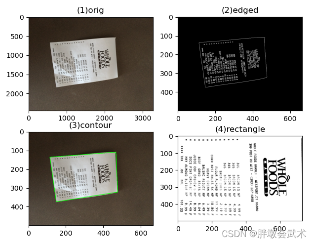
edged = cv2.Canny(gray, 75, 200) # Canny algorithm (edge detection)
##############################################
print("STEP 1: Edge Detection")
cv2.imshow("Image", image)
cv2.imshow("Edged", edged)
cv2.waitKey(0)
cv2.destroyAllWindows()
##############################################
# Profile Detection
cnts, hierarchy = cv2.findContours(edged.copy(), cv2.RETR_LIST, cv2.CHAIN_APPROX_SIMPLE)		# Profile Detection
cnts = sorted(cnts, key=cv2.contourArea, reverse=True)[:5] # Select the top five contours of all contours and sort them
for c in cnts:
peri = cv2.arcLength(c, True) # Calculate contour approximation
approx = cv2.approxPolyDP(c, 0.02 * peri, True) # find the polygonal fit curve of the contour
if len(approx) == 4: # If the current contour is four points (rectangles), then the current contour is the desired target.
screenCnt = approx
break
##############################################
print("STEP 2: Get Outline")
cv2.drawContours(image, [screenCnt], -1, (0, 255, 0), 2) # draw the detected contours on the original image
cv2.imshow("Outline", image)
cv2.waitKey(0)
cv2.destroyAllWindows()
##############################################
# Perspective transformations
warped = four_point_transform(orig, screenCnt.reshape(4, 2) * ratio) # get the outline to multiply by the scaled size of the image
warped = cv2.cvtColor(warped, cv2.COLOR_BGR2GRAY) # convert to grayscale
ref = cv2.threshold(warped, 100, 255, cv2.THRESH_BINARY)[1] # binary processing
ref = resize(ref, height=500)
##############################################
print("STEP 3: Chiral Transformation")
cv2.imshow("Scanned", ref)
cv2.waitKey(0)
cv2.destroyAllWindows()
##############################################
# The color channel for contour plotting is BGR; but Matplotlib is RGB; so when plotting, (0, 0, 255) will be converted from BGR to RGB (red - blue)
orig = cv2.cvtColor(orig, cv2.COLOR_BGR2RGB) # BGR to RGB conversion
edged = cv2.cvtColor(edged, cv2.COLOR_BGR2RGB)
image = cv2.cvtColor(image, cv2.COLOR_BGR2RGB)
ref = cv2.cvtColor(ref, cv2.COLOR_BGR2RGB)
plt.subplot(2, 2, 1),    plt.imshow(orig),      plt.title('orig')
plt.subplot(2, 2, 2),    plt.imshow(edged),     plt.title('edged')
plt.subplot(2, 2, 3),    plt.imshow(image),     plt.title('contour')
plt.subplot(2, 2, 4),    plt.imshow(ref),       plt.title('rectangle')
plt.show()
"""######################################################################
# Calculate the length of the curve: retval = cv2.arcLength(curve, closed)
# Input parameter: curve Contour (curve).
# closed If true, the outline is closed; if false, it is open. (Boolean type)
# Output parameters: retval The length (perimeter) of the contour.
######################################################################
# Find the polygonal fit curve of the contour: approxCurve = approxPolyDP(contourMat, 10, true)
# Input parameters: contourMat: contour point matrix (set)
# epsilon: (double type) the specified precision, i.e. the maximum distance between the original curve and the approximated curve.
# closed: (bool type) If true, the approximation curve is closed; conversely, if false, it is disconnected.
# Output parameters: approxCurve: contour point matrix (set); the current point set is the one that minimally accommodates the specified point set. The drawing is a polygon;
######################################################################"""
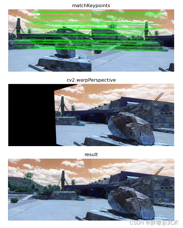
detectAndDescribe(), matchKeypoints(), cv2.findHomography(), cv2.warpPerspective(), drawMatches()
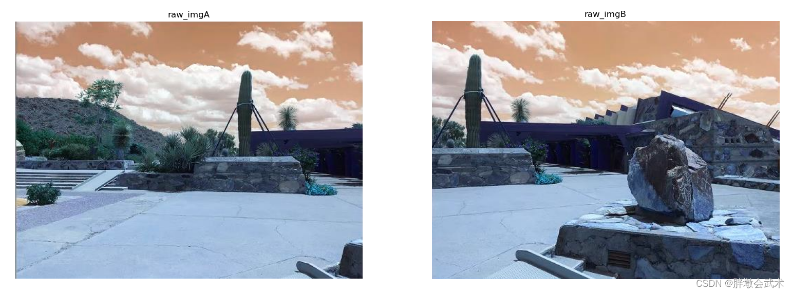
Function function: using the sift algorithm, implement the panoramic stitching algorithm, will be given two pictures spliced into one.
11:Detecting key points and extracting (sift) local invariant features from two input images.
22:Features between the two images matched (Lowe’s algorithm: comparing nearest neighbor distance to next nearest neighbor distance)
33:Estimation of the single mapping transformation matrix (homography: uni-responsiveness) using the RANSAC algorithm (Randomized Sampling Consistent Algorithm) with matching eigenvectors.
44:Apply a perspective transformation using the single-image matrix obtained from 33.
import cv2
import numpy as np
"""#########################################################
# Predefined framework descriptions
# Define a Stitcher class: stitch(), detectAndDescribe(), matchKeypoints(), drawMatches()
# stitch() stitch function
# detectAndDescribe() detects the SIFT key feature points of the image and computes the feature descriptors
# matchKeypoints() matches all the feature points of both images
# cv2.findHomography() computes the mono-mapping transformation matrix
# cv2.warpPerspective() Perspective transform (role: stitch image)
# drawMatches() builds a visualization of matches for straight line keypoints
#
# Note: cv2.warpPerspective() needs to be used with cv2.findHomography().
#########################################################"""
class Stitcher:
##################################################################################
def stitch(self, images, ratio=0.75, reprojThresh=4.0, showMatches=False):
(imageB, imageA) = images # Get the input images
(kpsA, featuresA) = self.detectAndDescribe(imageA) # Detect the SIFT key feature points of images A and B and compute the feature descriptors
(kpsB, featuresB) = self.detectAndDescribe(imageB)
M = self.matchKeypoints(kpsA, kpsB, featuresA, featuresB, ratio, reprojThresh) # Match all the feature points of the two images and return the match.
if M is None: # If the return result is null, there is no successful feature match, exit the algorithm
return None
# Otherwise, extract the match #
(matches, H, status) = M # H is the 3x3 view transformation matrix
result = cv2.warpPerspective(imageA, H, (imageA.shape[1] + imageB.shape[1], imageA.shape[0])) # transform image A into perspective, result is the transformed image
result[0: imageb.Shape [0], 0: imageb.shape [1]] = imageB # Passes imageB to the leftmost end of the result image
if showMatches: # Detect if you need to show image matches
vis = self.drawMatches(imageA, imageB, kpsA, kpsB, matches, status) # Generate matching images
return (result, vis)
return result
##################################################################################
def detectAndDescribe(self, image):
# gray = cv2.cvtColor(image, cv2.COLOR_BGR2GRAY) # Convert a color image to grayscale
descriptor = cv2.xfeatures2d.SIFT_create() # Create SIFT generator
"""#####################################################
# In case of OpenCV3.X, the cv2.xfeatures2d.SIFT_create method is used for DoG keypoint detection and SIFT feature extraction.
# In case of OpenCV 2.4, use cv2.FeatureDetector_create method for keypoint detection (DoG).
#####################################################"""
(kps, features) = descriptor.detectAndCompute(image, None) # detect SIFT feature points and compute descriptors
kps = np.float32([kp.pt for kp in kps]) # convert the result to a NumPy array
return (kps, features) # return the set of feature points, and the corresponding descriptive features
##################################################################################
def matchKeypoints(self, kpsA, kpsB, featuresA, featuresB, ratio, reprojThresh):
matcher = cv2.BFMatcher() # build the brute force matcher
rawMatches = matcher.knnMatch(featuresA, featuresB, 2) # Detect SIFT feature matching pairs from A and B graphs using KNN, K=2
matches = []
for m in rawMatches:
if len(m) == 2 and m[0].distance < m[1].distance * ratio: # keep the pair if the ratio of the closest distance to the next closest distance is less than the value of ratio
matches.append((m[0].trainIdx, m[0].queryIdx)) # store the indexes of the two points in featuresA, featuresB
if len(matches) > 4: # Calculate the perspective transformation matrix when the filtered matched pairs are greater than 4
# Projective transformation matrix: 3*3. has eight parameters corresponding to eight equations, one of which is 1 for normalization. Corresponds to four pairs, each pair (x, y)
ptsA = np.float32([kpsA[i] for (_, i) in matches]) # Get the coordinates of the points of the matched pairs
ptsB = np.float32([kpsB[i] for (i, _) in matches])
(H, status) = cv2.findHomography(ptsA, ptsB, cv2.RANSAC, reprojThresh) # Estimate the monoimage matrix using the RANSAC algorithm using the matching eigenvectors (homography: uni-responsiveness)
return (matches, H, status)
return None # If the pair is less than 4, return None.
##################################################################################
def drawMatches(self, imageA, imageB, kpsA, kpsB, matches, status):
(hA, wA) = imageA.shape[:2]
(hB, wB) = imageB.shape[:2]
vis = np.zeros((max(hA, hB), wA + wB, 3), dtype="uint8")
vis[0:hA, 0:wA] = imageA # Connect the left and right of the A and B maps together
vis[0:hB, wA:] = imageB
for ((trainIdx, queryIdx), s) in zip(matches, status):
if s == 1: # draw to visualization when point pair matching is successful
ptA = (int(kpsA[queryIdx][0]), int(kpsA[queryIdx][1]))
ptB = (int(kpsB[trainIdx][0]) + wA, int(kpsB[trainIdx][1]))
cv2.line(vis, ptA, ptB, (0, 255, 0), 1)
return vis # Return visualization results
##################################################################################
if __name__ == '__main__':
# Read the spliced images
imageA = cv2.imread("left_01.png")
imageB = cv2.imread("right_01.png")
# Stitching images into panoramas
stitcher = Stitcher() # call the splice function
(result, vis) = stitcher.stitch([imageA, imageB], showMatches=True)
# Show all images
cv2.imshow("Image A", imageA)
cv2.imshow("Image B", imageB)
cv2.imshow("Keypoint Matches", vis)
cv2.imshow("Result", result)
cv2.waitKey(0)
cv2.destroyAllWindows()
OpenCV based panoramic stitching (Python) SIFT/SURF
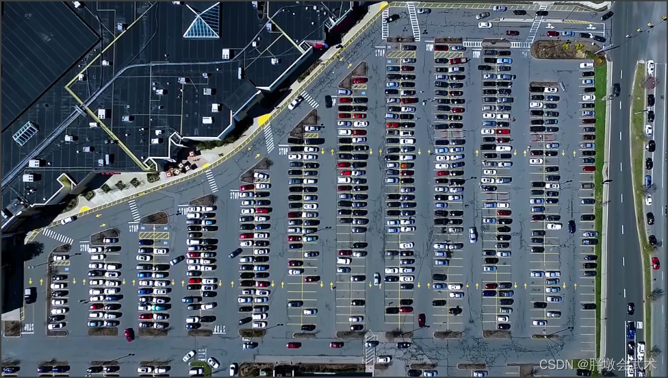
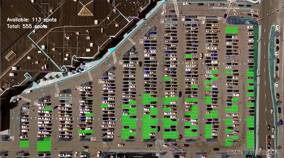
(iv) Parking lot space detection (Keras-based CNN classification) — pickle.dump(), pickle.load(), cv2.fillPoly(), cv2.bitwise_and(), cv2.circle(), cv2. HoughLinesP(), cv2.line()
The project is divided into three py files:Parking.py (defining all the functional functions), train.py (training the neural network), park_test.py (starting to detect the state of the parking space)
(1)Parking.py
#####################################################
# Parking.py
#####################################################
import matplotlib.pyplot as plt
import cv2
import os
import glob
import numpy as np
class Parking:
def show_images(self, images, cmap=None):
cols = 2
rows = (len(images)+1)//cols
plt.figure(figsize=(15, 12))
for i, image in enumerate(images):
plt.subplot(rows, cols, i+1)
cmap = 'gray' if len(image.shape) == 2 else cmap
plt.imshow(image, cmap=cmap)
plt.xticks([])
plt.yticks([])
plt.tight_layout(pad=0, h_pad=0, w_pad=0)
plt.show()
def cv_show(self, name, img):
cv2.imshow(name, img)
cv2.waitKey(0)
cv2.destroyAllWindows()
def select_rgb_white_yellow(self, image):
# Image background information filtering (i.e., intercept the image, specified range of colors)
lower = np.uint8([120, 120, 120])
upper = np.uint8([255, 255, 255])
# (1) lower_red and the portion above upper_red each becomes 0
# (2) The value between lower_red and upper_red becomes 255.
white_mask = cv2.inRange(image, lower, upper)
self.cv_show('white_mask', white_mask)
masked = cv2.bitwise_and(image, image, mask=white_mask)
self.cv_show('masked', masked)
return masked
def convert_gray_scale(self, image):
return cv2.cvtColor(image, cv2.COLOR_RGB2GRAY)
def detect_edges(self, image, low_threshold=50, high_threshold=200):
return cv2.Canny(image, low_threshold, high_threshold)
def filter_region(self, image, vertices):
# Functions: eliminates unwanted places, extracts polygons (positions of all parking spaces), pure white display
#####################################################
# zeros_like(array, dtype=float, order='C')
# Function: Returns a data of the given shape and type, filled with all zeros.
# Input parameters (1) array: input data
# (2) dtype: return the data type of the array (optional parameter, default float)
# (3) order: C for row first; F for column first (optional parameter)
#####################################################
mask = np.zeros_like(image) # new template (0: solid black)
if len(mask.shape) == 2:
#####################################################
# Fill arbitrary polygons: cv2.fillPoly(img, ppt, Scalar);
# Input Parameters (1) img Draws on this image.
# (2) ppt vertex sets of polygons
# (5) Scarlar Fill polygon color (255, 255, 255), i.e. RGB value is white
#####################################################
cv2.fillPoly(mask, vertices, 255) # fill polygon (255: pure white)
self.cv_show('mask', mask)
#####################################################
# cv2.bitwise_and() # bitwise and
# cv2.bitwise_or() # or
# cv2.bitwise_not() # not
# cv2.bitwise_xor() # hetero-ortho
###################################
# dst = cv2.bitwise_and(src1, src2, mask=mask)
# src1/src2 are images of the same type and size
# mask=mask indicates the area to be extracted (optional parameter)
# (1&1=1,1&0=0,0&1=0,0&0=0)
#####################################################
return cv2.bitwise_and(image, mask) # bitwise and operation
def select_region(self, image):
# Function: (Manual) Select Area - In the original drawing, filter out the locations of all parking spaces and frame them into a polygon.
# Polygon keypoint positions are set by customization as follows.
rows, cols = image.shape[:2] # Get the length and width of the image
pt_1 = [cols*0.05, rows*0.90] # position point 1
pt_2 = [cols*0.05, rows*0.70] # position point 2
pt_3 = [cols*0.30, rows*0.55] # position point 3
pt_4 = [cols*0.6, rows*0.15] # position point 4
pt_5 = [cols*0.90, rows*0.15] # position point 5
pt_6 = [cols*0.90, rows*0.90] # position point 6
vertices = np.array([[pt_1, pt_2, pt_3, pt_4, pt_5, pt_6]], dtype=np.int32) # convert the data to a numpy array
point_img = image.copy()
point_img = cv2.cvtColor(point_img, cv2.COLOR_GRAY2RGB) # convert to grayscale
for point in vertices[0]: # Iterate over all position points
"""#####################################################
# Draw circle shape: cv2.circle(image, center, radius, color, thickness)
# Input Parameters (1) Image: Plot on this image.
# (2) Circle center: The coordinates of the center of the circle. The coordinates are represented as a tuple of two values, i.e. (X coordinate value, Y coordinate value).
# (3) Radius: the radius of a circle.
# (4) Color: The color of the circle's boundary line. For BGR, we pass a tuple. For example: (255, 0, 0) for blue color.
# (5) Thickness: A positive number indicates the thickness of the line. Where: -1 indicates a solid circle.
#####################################################"""
cv2.circle(point_img, (point[0], point[1]), 10, (0, 0, 255), 4) # draw a hollow circle at each position point
self.cv_show('point_img', point_img)
return self.filter_region(image, vertices)
def hough_lines(self, image):
"""#####################################################
# Detect all lines in the image: cv2.HoughLinesP(image, rho=0.1, theta=np.pi / 10, threshold=15, minLineLength=9, maxLineGap=4)
# image The input image needs to be the result of edge detection
# minLineLengh (the shortest length of the line, anything shorter than this is ignored)
# MaxLineCap (the maximum spacing between two lines, less than which a line is considered to be a straight line)
# rho distance accuracy
# theta angular accuracy
# threshod exceeds the set threshold to be detected as a line segment
#####################################################"""
return cv2.HoughLinesP(image, rho=0.1, theta=np.pi/10, threshold=15, minLineLength=9, maxLineGap=4)
def draw_lines(self, image, lines, color=[255, 0, 0], thickness=2, make_copy=True):
# Function: Draw all lines on the original drawing that satisfy the condition
if make_copy:
image = np.copy(image)
cleaned = []
for line in lines:
for x1, y1, x2, y2 in line: # A line consists of two points, each with coordinates (x, y)
# abs(y2-y1) <= 1 ---- The images are all straight lines with slopes converging to 0
# abs(x2-x1) >= 25 and abs(x2-x1) <= 55 ---- Line Segment Custom Filtering (set up as appropriate)
if abs(y2-y1) <= 1 and abs(x2-x1) >= 25 and abs(x2-x1) <= 55:
cleaned.append((x1, y1, x2, y2)) # save all lines that satisfy the condition
cv2.line(image, (x1, y1), (x2, y2), color, thickness) # on the original image, draw all lines that satisfy the condition
print(" No lines detected: ", len(cleaned))
return image
def identify_blocks(self, image, lines, make_copy=True):
#####################################################
# Function: Recognizes all parking spaces
# Step 1: Filter some of the straight lines and extract the valid ones (i.e. the ones corresponding to the parking spaces)
# Step 2: Sorting Straight Lines
# Step 3: Find multiple columns, each corresponding to a row of cars
# Step 4: Get the coordinates of each column of rectangles
# Step 5: Draw the column rectangles out
#####################################################
if make_copy:
new_image = np.copy(image)
# Step 1: Filter some of the straight lines and extract the valid ones (i.e. the ones corresponding to the parking spaces)
cleaned = []
for line in lines:
for x1, y1, x2, y2 in line:
if abs(y2-y1) <=1 and abs(x2-x1) >=25 and abs(x2-x1) <= 55:
cleaned.append((x1, y1, x2, y2)) # save all lines that satisfy the condition
# Step 2: Sorting Straight Lines
import operator
list1 = sorted(cleaned, key=operator.itemgetter(0, 1)) # label all lines with order (sort: top to bottom, left to right)
# Step 3: Find multiple columns, each corresponding to a row of cars
clusters = {} # find all lines in the same column
dIndex = 0
clus_dist = 10 # Distance between column and nearest column (set as appropriate)
for i in range(len(list1) - 1):
distance = abs(list1[i+1][0] - list1[i][0])
if distance <= clus_dist:
if not dIndex in clusters.keys(): clusters[dIndex] = []
clusters[dIndex].append(list1[i])
clusters[dIndex].append(list1[i + 1])
else:
dIndex += 1 # Summarize lines in same column, otherwise skip
# Step 4: Get the coordinates of each column of rectangles
rects = {}
i = 0
for key in clusters: column # 12
all_list = clusters[key]
cleaned = list(set(all_list))
if len(cleaned) > 5: # If the number is greater than 5, define it as a column
cleaned = sorted(cleaned, key=lambda tup: tup[1])
avg_y1 = cleaned[0][1] # Extract the first line of each column.        [0] indicates the first line
avg_y2 = cleaned[-1][1] # Extract the last line of each column [-1] means last line
avg_x1 = 0 # Take the mean value since the x's of the different lines are not uniformly hierarchical
avg_x2 = 0
for tup in cleaned:
avg_x1 += tup[0]
avg_x2 += tup[2]
avg_x1 = avg_x1/len(cleaned) # x1 is the start of the rectangle
avg_x2 = avg_x2/len(cleaned) # x2 is the termination point of the rectangle
rects[i] = (avg_x1, avg_y1, avg_x2, avg_y2) # get the four point coordinates of each column of rectangles
i += 1
print("Num Parking Lanes: ", len(rects)) # There are 12 rectangles in total
# Step 5: Draw the column rectangles out
buff = 7
for key in rects: # key indicates the number of columns
tup_topLeft = (int(rects[key][0] - buff), int(rects[key][1]))
tup_botRight = (int(rects[key][2] + buff), int(rects[key][3]))
cv2.rectangle(new_image, tup_topLeft, tup_botRight, (0, 255, 0), 3)
return new_image, rects
def draw_parking(self, image, rects, make_copy=True, color=[255, 0, 0], thickness=2, save=True):
if make_copy:
new_image = np.copy(image)
gap = 15.5 # Fix the distance interval between every two parking spaces (y-axis)
spot_dict = {} # Dictionary: one space corresponds to one location
tot_spots = 0
# Fine-tuning --- Since the detected rectangles have a certain degree of error, human manipulation is performed to achieve precision
adj_y1 = {0: 20, 1: -10, 2: 0, 3: -11, 4: 28, 5: 5, 6: -15, 7: -15, 8: -10, 9: -30, 10: 9, 11: -32}
adj_y2 = {0: 30, 1: 50, 2: 15, 3: 10, 4: -15, 5: 15, 6: 15, 7: -20, 8: 15, 9: 15, 10: 0, 11: 30}
adj_x1 = {0: -8, 1: -15, 2: -15, 3: -15, 4: -15, 5: -15, 6: -15, 7: -15, 8: -10, 9: -10, 10: -10, 11: 0}
adj_x2 = {0: 0, 1: 15, 2: 15, 3: 15, 4: 15, 5: 15, 6: 15, 7: 15, 8: 10, 9: 10, 10: 10, 11: 0}
for key in rects: # key indicates the number of columns
tup = rects[key]
x1 = int(tup[0] + adj_x1[key])
x2 = int(tup[2] + adj_x2[key])
y1 = int(tup[1] + adj_y1[key])
y2 = int(tup[3] + adj_y2[key])
cv2.rectangle(new_image, (x1, y1), (x2, y2), (0, 255, 0), 2) # draw the fine-tuned rectangle on the image
num_splits = int(abs(y2-y1)//gap) # Calculate how many cars can be parked in each column on average (averaging estimate due to errors that do not identify exact parking spaces)
for i in range(0, num_splits+1): # Cutting six cuts gives seven parking spaces
y = int(y1 + i*gap)
#####################################################
Draw a straight line: cv2.line(img, pt1, pt2, color, thickness)
# Input parameter img The image where the line to be drawn is located.
# pt1 Straight line starting point
# pt2 Straight end
# color The color of the straight line
thickness=1 line thickness
#####################################################
# Draw the horizontal lines of all parking spaces
cv2.line(new_image, (x1, y), (x2, y), color, thickness)
if 0 < key < len(rects) - 1: # The first and last columns are single rows, the rest are double rows (depending on the situation).
# Draw vertical lines between double rows of parking spaces #
x = int((x1 + x2)/2) # The midpoint of the two locations is the corresponding vertical line coordinates
cv2.line(new_image, (x, y1), (x, y2), color, thickness)
# of calculations
if key == 0 or key == (len(rects) - 1): # If it's a single-row parking space, just +1 it.
tot_spots += num_splits + 1
else: # If it's a double row of parking spaces, +1, then multiply by 2.
tot_spots += 2*(num_splits + 1)
# One-to-one key-value pairs for each parking space with a dictionary
if key == 0 or key == (len(rects) - 1): # First or last column (single row parking)
for i in range(0, num_splits+1):
cur_len = len(spot_dict)
y = int(y1 + i*gap)
spot_dict[(x1, y, x2, y+gap)] = cur_len + 1 # Coordinates of the first and last parking spot columns
else: # double rows of parking spaces
for i in range(0, num_splits+1):
cur_len = len(spot_dict)
y = int(y1 + i*gap)
x = int((x1 + x2)/2) # Midpoint position corresponding to double row of parking spaces
spot_dict[(x1, y, x, y+gap)] = cur_len + 1 # Coordinates of the left row of a double row of parking spaces
spot_dict[(x, y, x2, y+gap)] = cur_len + 2 # Coordinates of the right row of a double row of parking spaces
print("total parking spaces: ", tot_spots, cur_len)
if save:
filename = 'with_parking.jpg'
cv2.imwrite(filename, new_image)
return new_image, spot_dict
def assign_spots_map(self, image, spot_dict, make_copy=True, color=[255, 0, 0], thickness=2):
if make_copy:
new_image = np.copy(image)
for spot in spot_dict.keys():
(x1, y1, x2, y2) = spot
cv2.rectangle(new_image, (int(x1), int(y1)), (int(x2), int(y2)), color, thickness)
return new_image
def save_images_for_cnn(self, image, spot_dict, folder_name='cnn_data'):
# Function: crop the parking spaces to get the images corresponding to all the parking spaces and save them under the specified folder path. (Provide data for CNN training. The images need to be manually filtered into two categories before training: whether the parking space is occupied or not.)
for spot in spot_dict.keys(): # Iterate over all parking spots -- indexed by the dictionary's keys
(x1, y1, x2, y2) = spot
(x1, y1, x2, y2) = (int(x1), int(y1), int(x2), int(y2))) # Coordinate values are rounded
spot_img = image[y1:y2, x1:x2] # crop the parking space
spot_img = cv2.resize(spot_img, (0, 0), fx=2.0, fy=2.0) # image crop (original image is in too mini)
spot_id = spot_dict[spot] # Coordinates of the parking space - the value corresponding to the key
filename = 'spot' + str(spot_id) + '.jpg' # Name each parking space with a key (so that subsequent indexing requirements can be followed)
print(spot_img.shape, filename, (x1, x2, y1, y2))
cv2.imwrite(os.path.join(folder_name, filename), spot_img) # save the parking spot image to the specified folder (cnn_data) path
def make_prediction(self, image, model, class_dictionary):
# Pre-processing
img = image/255.
# Converted to 4D tensor
image = np.expand_dims(img, axis=0)
# Train with a trained model
class_predicted = model.predict(image)
inID = np.argmax(class_predicted[0])
label = class_dictionary[inID]
return label
def predict_on_image(self,image, spot_dict , model,class_dictionary,make_copy=True, color=[0, 255, 0], alpha=0.5):
if make_copy:
new_image = np.copy(image)
overlay = np.copy(image)
self.cv_show('new_image', new_image)
cnt_empty = 0
all_spots = 0
for spot in spot_dict.keys():
all_spots += 1
(x1, y1, x2, y2) = spot
(x1, y1, x2, y2) = (int(x1), int(y1), int(x2), int(y2))
spot_img = image[y1:y2, x1:x2]
spot_img = cv2.resize(spot_img, (48, 48))
label = self.make_prediction(spot_img,model,class_dictionary) # Predict whether the image (parking space) is occupied or not
if label == 'empty':
cv2.rectangle(overlay, (int(x1), int(y1)), (int(x2), int(y2)), color, -1)
cnt_empty += 1
cv2.addWeighted(overlay, alpha, new_image, 1-alpha, 0, new_image) # Image fusion
cv2.putText(new_image, "Available: %d spots" % cnt_empty, (30, 95), cv2.FONT_HERSHEY_SIMPLEX, 0.7, (255, 255, 255), 2)
cv2.putText(new_image, "Total: %d spots" % all_spots, (30, 125), cv2.FONT_HERSHEY_SIMPLEX, 0.7, (255, 255, 255), 2)
save = False
if save:
filename = 'with_marking.jpg'
cv2.imwrite(filename, new_image)
self.cv_show('new_image', new_image)
return new_image
def predict_on_video(self, video_name, final_spot_dict, model, class_dictionary, ret=True):
cap = cv2.VideoCapture(video_name)
count = 0
while ret:
ret, image = cap.read()
count += 1
if count == 5: # Judge every four images
count = 0
new_image = np.copy(image)
overlay = np.copy(image)
cnt_empty = 0
all_spots = 0
color = [0, 255, 0]
alpha = 0.5
for spot in final_spot_dict.keys():
all_spots += 1
(x1, y1, x2, y2) = spot
(x1, y1, x2, y2) = (int(x1), int(y1), int(x2), int(y2))
spot_img = image[y1:y2, x1:x2]
spot_img = cv2.resize(spot_img, (48,48))
label = self.make_prediction(spot_img, model, class_dictionary) # Predict whether the frame image (parking space) is occupied or not
if label == 'empty':
cv2.rectangle(overlay, (int(x1), int(y1)), (int(x2), int(y2)), color, -1)
cnt_empty += 1
cv2.addWeighted(overlay, alpha, new_image, 1 - alpha, 0, new_image)
cv2.putText(new_image, "Available: %d spots" % cnt_empty, (30, 95), cv2.FONT_HERSHEY_SIMPLEX, 0.7, (255, 255, 255), 2)
cv2.putText(new_image, "Total: %d spots" % all_spots, (30, 125), cv2.FONT_HERSHEY_SIMPLEX, 0.7, (255, 255, 255), 2)
cv2.imshow('frame', new_image)
if cv2.waitKey(10) & 0xFF == ord('q'):
break
cv2.destroyAllWindows()
cap.release()
(2)train.py
#####################################################
# train.py
#####################################################
import numpy
import os
from keras import applications
from keras.preprocessing.image import ImageDataGenerator
from keras import optimizers
from keras.models import Sequential, Model
from keras.layers import Dropout, Flatten, Dense, GlobalAveragePooling2D
from keras import backend as k
from keras.callbacks import ModelCheckpoint, LearningRateScheduler, TensorBoard, EarlyStopping
from keras.models import Sequential
from keras.layers.normalization import BatchNormalization
from keras.layers.convolutional import Conv2D
from keras.layers.convolutional import MaxPooling2D
from keras.initializers import TruncatedNormal
from keras.layers.core import Activation
from keras.layers.core import Flatten
from keras.layers.core import Dropout
from keras.layers.core import Dense
files_train = 0
files_validation = 0
########################################
cwd = os.getcwd() # Get the current working path
folder = 'train_data/train' # Training data
for sub_folder in os.listdir(folder):
path, dirs, files = next(os.walk(os.path.join(folder, sub_folder))) # Read data
files_train += len(files)
########################################
folder = 'train_data/test' # Test data
for sub_folder in os.listdir(folder):
path, dirs, files = next(os.walk(os.path.join(folder, sub_folder))) # Read data
files_validation += len(files)
########################################
print(files_train, files_validation)
########################################
# CNN training parameters specified
img_width, img_height = 48, 48
train_data_dir = "train_data/train"
validation_data_dir = "train_data/test"
nb_train_samples = files_train
nb_validation_samples = files_validation
batch_size = 32
epochs = 15
num_classes = 2
# Call the VGG16 network in applications in the kera framework. Several network models are encapsulated in there (VGG16, VGG19, Resnet50, MobileNet, etc.)
# weights='imagenet' means call imagenet-trained weights directly (current data is too small)
model = applications.VGG16(weights='imagenet', include_top=False, input_shape=(img_width, img_height, 3))
########################################
# Freeze the first 10 layers of the network #
for layer in model.layers[:10]:
layer.trainable = False
x = model.output
x = Flatten()(x)
predictions = Dense(num_classes, activation="softmax")(x)
model_final = Model(input=model.input, output=predictions)
model_final.compile(loss="categorical_crossentropy", optimizer = optimizers.SGD(lr=0.0001, momentum=0.9), metrics=["accuracy"])
########################################
# Data enhancement
train_datagen = ImageDataGenerator(rescale=1./255, horizontal_flip=True, fill_mode="nearest",
zoom_range=0.1, width_shift_range=0.1, height_shift_range=0.1, rotation_range=5)
test_datagen = ImageDataGenerator(rescale=1./255, horizontal_flip=True, fill_mode="nearest",
zoom_range=0.1, width_shift_range=0.1, height_shift_range=0.1, rotation_range=5)
train_generator = train_datagen.flow_from_directory(train_data_dir, target_size=(img_height, img_width), batch_size=batch_size, class_mode="categorical")
validation_generator = test_datagen.flow_from_directory(validation_data_dir, target_size=(img_height, img_width), class_mode="categorical")
########################################
checkpoint = ModelCheckpoint("car1.h5", monitor='val_acc', verbose=1, save_best_only=True, save_weights_only=False, mode='auto', period=1)
early = EarlyStopping(monitor='val_acc', min_delta=0, patience=10, verbose=1, mode='auto')
history_object = model_final.fit_generator(train_generator, samples_per_epoch=nb_train_samples, epochs=epochs,
validation_data=validation_generator, nb_val_samples=nb_validation_samples, callbacks=[checkpoint, early])
# Files are automatically generated after training: car1.h5
# Note: The final training result is only ninety percent. (1) There is still room for improvement in data preprocessing (2) The neural network model can be optimized
(3)park_test.py
#####################################################
# park_test.py
#####################################################
from __future__ import division
import matplotlib.pyplot as plt
import cv2
import os
import glob
import numpy as np
from keras.applications.imagenet_utils import preprocess_input
from keras.models import load_model
from keras.preprocessing import image
from PIL import Image
# Pillow (PIL) is a more basic image processing library in Python, mainly used for basic image processing, such as cropping images, resizing images and image color processing.
# Compared with Pillow, OpenCV and Scikit-image are more feature-rich and therefore more complex to use, and are mainly used in machine vision and image analysis, such as the well-known "face recognition" applications.
import pickle
from Parking import Parking # Import a custom library
cwd = os.getcwd()
def img_process(test_images, park): # park: instantiated class
white_yellow_images = list(map(park.select_rgb_white_yellow, test_images)) # select_rgb_white_yellow(): filters image background information
park.show_images(white_yellow_images)
########################################################################################################
gray_images = list(map(park.convert_gray_scale, white_yellow_images)) # convert_gray_scale(): Convert to grayscale
park.show_images(gray_images)
########################################################################################################
edge_images = list(map(lambda image: park.detect_edges(image), gray_images)) # detect_edges(): Use the cv2.Canny algorithm for edge detection
park.show_images(edge_images)
########################################################################################################
roi_images = list(map(park.select_region, edge_images)) # select_region(): filter out polygons (parking lot locations) and remove redundant regions from the image
park.show_images(roi_images)
########################################################################################################
list_of_lines = list(map(park.hough_lines, roi_images)) # hough_lines(): detect all lines in the image
########################################################################################################
line_images = []
for image, lines in zip(test_images, list_of_lines):
line_images.append(park.draw_lines(image, lines)) # draw_lines(): draw all lines in the image that satisfy the condition (i.e. parking lines)
park.show_images(line_images)
########################################################################################################
rect_images = [] # new_image draws the image with all rectangles
rect_coords = [] # rects The coordinates of the four points of each rectangle.
for image, lines in zip(test_images, list_of_lines):
new_image, rects = park.identify_blocks(image, lines) # identify_blocks(): Draw rectangles for each column
rect_images.append(new_image)
rect_coords.append(rects)
park.show_images(rect_images) # draw (rectangular) images
########################################################################################################
delineated = [] # new_image draws an image with all rectangles after delineation, and all parking spaces
spot_pos = [] # spot_dict Coordinates of each parking space (dictionary - data structure)
for image, rects in zip(test_images, rect_coords):
new_image, spot_dict = park.draw_parking(image, rects) # draw_parking: Draw the parking space
delineated.append(new_image)
spot_pos.append(spot_dict)
park.show_images(delineated) # draw (rectangle + parking space) images
final_spot_dict = spot_pos[1] # Fetch all values of the dictionary (key-value pairs) (each value corresponds to the coordinate position of a parking spot). [1]: values
print(len(final_spot_dict)) # print all parking spots
########################################################################################################
with open('spot_dict.pickle', 'wb') as handle: # Open the file (open) and close it automatically (with)
"""#####################################################
# The pickle module in Python implements basic data serialization and deserialization. Serializing an object allows you to save the object on disk and read it out when needed. Any object can perform serialization operations.
#####################################################
# (1) serialize-archive: pickle.dump(obj, file, protocol)
# Input parameters Object: that's what you're storing, the type can be list, string and any other type
# File: This is the destination file where the object will be stored.
# Protocols used: 3, index 0 is ASCII (default), 1 is old-style binary, 2 is new-style binary protocols
#       fw = open("pickleFileName.txt", "wb")
#       pickle.dump("try", fw)
#####################################################
# (2) Deserialize-read file: pickle.load(file)
#       fr = open("pickleFileName.txt", "rb")
#       result = pickle.load(fr)
#####################################################"""
pickle.dump(final_spot_dict, handle, protocol=pickle.HIGHEST_PROTOCOL) # Save the current preprocessing result and call it directly later.
########################################################################################################
park.save_images_for_cnn(test_images[0], final_spot_dict) # save_images_for_cnn(): call CNN neural network to recognize if the parking space is occupied or not
return final_spot_dict
########################################################################################################
def keras_model(weights_path):
# from keras.models import load_model
model = load_model(weights_path) # load_model() car1.h5 (model generated after neural network training)
return model
def img_test(test_images, final_spot_dict, model, class_dictionary):
for i in range(len(test_images)):
predicted_images = park.predict_on_image(test_images[i], final_spot_dict, model, class_dictionary)
# predict_on_image():
def video_test(video_name, final_spot_dict, model, class_dictionary):
name = video_name
cap = cv2.VideoCapture(name)
park.predict_on_video(name, final_spot_dict, model, class_dictionary, ret=True)
if __name__ == '__main__':
# Folder name: test_images
test_images = [plt.imread(path) for path in glob.glob('test_images/*.jpg')]
weights_path = 'car1.h5'
video_name = 'parking_video.mp4'
# class_dictionary = {0: 'empty', 1: 'occupied'} # Occupied parking space
class_dictionary = {} # Parking space occupancy status
class_dictionary[0] = 'empty' # Car parking space is empty
class_dictionary[1] = 'occupied' # Occupied
park = Parking() # Instantiation of class
park.show_images(test_images)
final_spot_dict = img_process(test_images, park) # Image preprocessing
model = keras_model(weights_path) # load neural network trained model
img_test(test_images, final_spot_dict, model, class_dictionary)
video_test(video_name, final_spot_dict, model, class_dictionary)
Introduction to 8 Mainstream Deep Learning Frameworks
The PIL Library in Python
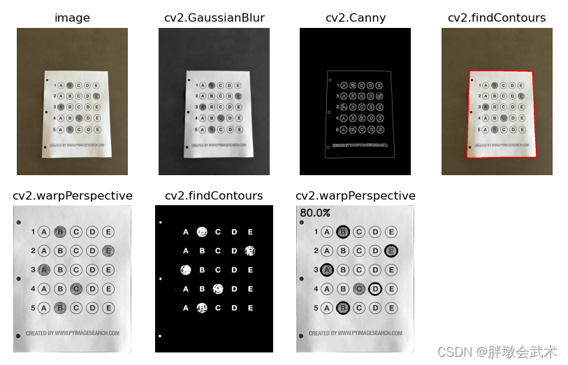
(v) Answer key recognition and marking — cv2.putText(), cv2.countNonZero()
import cv2 # opencv reads in BGR format
import numpy as np
import matplotlib.pyplot as plt # Matplotlib is RGB
def order_points(pts):
# There are four coordinate points
rect = np.zeros((4, 2), dtype="float32")
# Find the coordinates 0123 in order # - Upper left, upper right, lower right, lower left.
# Calculate top left, bottom right
s = pts.sum(axis=1)
rect[0] = pts[np.argmin(s)]
rect[2] = pts[np.argmax(s)]
# Calculate upper right and lower left
diff = np.diff(pts, axis=1)
rect[1] = pts[np.argmin(diff)]
rect[3] = pts[np.argmax(diff)]
return rect
def four_point_transform(image, pts):
# Get input coordinate points
rect = order_points(pts)
(tl, tr, br, bl) = rect
# Calculate the input w and h values
widthA = np.sqrt(((br[0] - bl[0]) ** 2) + ((br[1] - bl[1]) ** 2))
widthB = np.sqrt(((tr[0] - tl[0]) ** 2) + ((tr[1] - tl[1]) ** 2))
maxWidth = max(int(widthA), int(widthB))
heightA = np.sqrt(((tr[0] - br[0]) ** 2) + ((tr[1] - br[1]) ** 2))
heightB = np.sqrt(((tl[0] - bl[0]) ** 2) + ((tl[1] - bl[1]) ** 2))
maxHeight = max(int(heightA), int(heightB))
# Transformed coordinate positions
dst = np.array([[0, 0], [maxWidth - 1, 0], [maxWidth - 1, maxHeight - 1], [0, maxHeight - 1]], dtype="float32")
# Calculate the transformation matrix
M = cv2 getPerspectiveTransform (the rect, DST) # : calculate the homogeneous transformation matrix cv2. GetPerspectiveTransform (DST) the rect,
warped = cv2.warpPerspective(image, M, (maxWidth, maxHeight)) # Perspective transform: (multiply input rectangle by (chi-square transform matrix) to get output matrix)
return warped
def sort_contours(cnts, method="left-to-right"):
reverse = False
i = 0
if method == "right-to-left" or method == "bottom-to-top":
reverse = True
if method == "top-to-bottom" or method == "bottom-to-top":
i = 1
boundingBoxes = [cv2.boundingRect(c) for c in cnts]
(cnts, boundingBoxes) = zip(*sorted(zip(cnts, boundingBoxes), key=lambda b: b[1][i], reverse=reverse))
return cnts, boundingBoxes
"""#############################################################
# if __name__ == '__main__':
# (1) "__name__" is a built-in Python variable that refers to the current module.
# (2) The value of "__name__" of a module is "__main__" when that module is directly executed.
# (3) When imported into another module, the value of "__name__" is the real name of the module.
#############################################################"""
# Need to be given the correct answer for the option corresponding to each image (dictionary: keys correspond to rows, values correspond to answers for each row)
ANSWER_KEY = {0: 1, 1: 4, 2: 0, 3: 3, 4: 1}
# Image preprocessing
image = cv2.imread(r"images/test_01.png")
contours_img = image.copy()
gray = cv2.cvtColor(image, cv2.COLOR_BGR2GRAY) # Convert to gray scale image
blurred = cv2.GaussianBlur(gray, (5, 5), 0) # Gaussian filter - removes noise
edged = cv2.Canny(blurred, 75, 200) # Canny operator edge detection
cnts, hierarchy = cv2.findContours(edge.copy (), cv2.RETR_EXTERNAL, cv2.CHAIN_APPROX_SIMPLE) # profile detection
Cv2. DrawContours (contours_img, CNTS, 1, (0, 0, 255), 3) # draw the contour (sheet)
###################################################################
# Extracting the answer key and making perspective changes
docCnt = None
if len(cnts) > 0:
cnts = sorted(cnts, key=cv2.contourArea, reverse=True) # sort by contour size
for c in cnts: # iterate over each contour
peri = cv2.arcLength(c, True) # Calculate the length of the outline
approx = cv2.approxPolyDP(c, 0.02*peri, True) # find the polygonal fit curve of the contour
if len(approx) == 4: # the found outline is a quadrilateral (corresponding to four vertices)
docCnt = approx
break
warped = four_point_transform(gray, docCnt.reshape(4, 2)) # Perspective transform (chi-square transform matrix)
warped1 = warped.copy()
thresh = cv2.threshold(warped, 0, 255, cv2.THRESH_BINARY_INV | cv2.THRESH_OTSU)[1] # 0: means the system determines it automatically; THRESH_OTSU: adaptive threshold setting
###############################
thresh_Contours = thresh.copy()
cnts, hierarchy = cv2.findContours(thresh.copy(), cv2.RETR_EXTERNAL, cv2.CHAIN_APPROX_SIMPLE) # find each circle outline
Cv2. DrawContours (thresh_Contours, CNTS, 1, (0, 0, 255), 3) # draw all contours
###################################################################
# Extract all valid choices in the answer key (circle)
questionCnts = [] # Extract the outline of each option
for c in cnts:
(x, y, w, h) = cv2.boundingRect(c) # Get the dimensions of the outline
ar = w / float(h) # Calculate the ratio
if w >= 20 and h >= 20 and 0.9 <= ar <= 1.1: # Customize the set size (as appropriate)
questionCnts.append(c)
questionCnts = sort_contours(questionCnts, method="top-to-bottom")[0] # Sort all options from top to bottom
###############################
correct = 0
for (q, i) in enumerate(np.arange(0, len(questionCnts), 5)): # There are 5 options per row
cnts = sort_contours(questionCnts[i:i + 5])[0] # sort for each row
bubbled = None
for (j, c) in enumerate(cnts): # iterate over the five results corresponding to each row
mask = np.zeros(thresh.shape, dtype="uint8") # use mask to determine the result (all black: 0) indicating that the scribbled answer is correct
Cv2. DrawContours (mask, [c], 1, 255, 1) # 1 said filling
# cv_show('mask', mask) # Show each option
mask = cv2.bitwise_and(thresh, thresh, mask=mask) # mask=mask indicates the region to extract (optional parameter)
total = cv2.countNonZero(mask) # count whether to choose this answer by counting the number of nonzero points
if bubbled is None or total > bubbled[0]: # Record the maximum number
bubbled = (total, j)
color = (0, 0, 255) # Compare to the correct answer.
k = ANSWER_KEY[q]
# The judgment is right
if k == bubbled[1]:
color = (0, 255, 0)
correct += 1
cv2.drawContours(warped, [cnts[k]], -1, color, 3) # Draw the outline
###################################################################
# Show results
score = (correct / 5.0) * 100 # Calculate total score
print("[INFO] score: {:.2f}%".format(score))
"""###################################################################
# Add text content to the image: cv2.putText(img, str(i), (123,456), cv2.FONT_HERSHEY_PLAIN, 2, (0,255,0), 3)
# The parameters are, in order: image, added text, top-left corner coordinates, font type, font size, color, font thickness
# Added font: "{:.2f}%".format(score) ---- means add the score string. And keep all the integer bits and two decimal places.
###################################################################"""
cv2.putText(warped, "{:.1f}%".format(score), (10, 30), cv2.FONT_HERSHEY_SIMPLEX, 0.9, (0, 0, 255), 2)
image = cv2.cvtColor(image, cv2.COLOR_BGR2RGB) # opencv reads in BGR format, Matplotlib in RGB
contours_img = cv2.cvtColor(contours_img, cv2.COLOR_BGR2RGB)
plt.subplot(241),       plt.imshow(image, cmap='gray'),         	plt.axis('off'),    plt.title('image')
plt.subplot(242),       plt.imshow(blurred, cmap='gray'),       	plt.axis('off'),    plt.title('cv2.GaussianBlur')
plt.subplot(243),       plt.imshow(edged, cmap='gray'),         	plt.axis('off'),    plt.title('cv2.Canny')
plt.subplot(244),       plt.imshow(contours_img, cmap='gray'),      plt.axis('off'),    plt.title('cv2.findContours')
plt.subplot(245),       plt.imshow(warped1, cmap='gray'),        	plt.axis('off'),    plt.title('cv2.warpPerspective')
plt.subplot(246),       plt.imshow(thresh_Contours, cmap='gray'),   plt.axis('off'),    plt.title('cv2.findContours')
plt.subplot(247),       plt.imshow(warped, cmap='gray'),        	plt.axis('off'),    plt.title('cv2.warpPerspective')
plt.show()
(vi) Background modeling (dynamic target recognition) — cv2.getStructuringElement(), cv2.createBackgroundSubtractorMOG2()
"""########################################################
# Background modeling (detection of moving targets)
# Method I: frame difference method
# Introduction: as the target in the scene is moving, the image of the target has different positions in different image frames.
# (1) This class of algorithms performs a difference operation on two temporally consecutive image frames, where the pixel points corresponding to different frames are subtracted to determine the absolute value of the gray level difference.
# (2) When the absolute value exceeds a certain threshold, it can be judged as a moving target, thus realizing the target detection function.
# Advantages and disadvantages: the frame difference method is very simple, but introduces noise and nulling problems
# Method II: Hybrid Gaussian modeling
# Introduction: (1) Background training, each background in the image is simulated using a [mixed Gaussian model], and the number of mixed Gaussians for each background can be adaptive.
# (2) In the testing phase, a GMM match is performed on the incoming pixel, and if the pixel value can match one of the Gaussians, it is considered to be the background, otherwise it is considered to be the foreground.
# Feature 1: The GMM model is robust to dynamic backgrounds since the whole process is under continuous update learning.
# Feature 2: For the variation of pixel points in the video should be consistent with a Gaussian distribution, the actual distribution of the background should be a mixture of multiple Gaussian distributions, and each Gaussian model can also be weighted.
# Hybrid Gaussian model learning methods
# 1. First initialize each Gaussian model matrix parameter.
# 2.Take T frames of image data from the video used to train the Gaussian mixture model and take the first pixel as the first Gaussian distribution.
# 3. Subsequent pixel values are compared to the mean of the previous Gaussian distribution and if the difference is within 3 times the variance, they belong to the same Gaussian distribution and their parameters are updated. Otherwise a new Gaussian distribution is created with this pixel.
# Hybrid Gaussian model test methods
# In the test phase, the value of the incoming pixel point is compared to each mean value in the hybrid Gaussian model and is considered as background if the difference is between 2 times the variance, otherwise it is considered as foreground (dynamic target).
# Assign the foreground to 255 and the background to 0. This creates a foreground binary map.
########################################################"""
import cv2
cap = cv2.VideoCapture('test.avi') # Capture camera
"""########################################################
# constructs convolution kernels: cv2. GetStructuringElement (shape, ksize, anchor = None)
# Input parameters shape: (1) Enumerator
# (2) MORPH_RECT Rectangle
# (3) MORPH_CROSS Cross-shaped
# (4) MORPH_ELLIPSE ellipsoidal
# ksize: convolution kernel size (tuple type) e.g. (3, 4)
# anchor: the position of the stroke inside the element, defaults to (-1, -1) indicating the center of the shape
# Prerequisites: background is black, value 0, object is white, value 1
########################################################"""
kernel = cv2.getStructuringElement(cv2.MORPH_ELLIPSE, (3, 3)) # Required for morphological operations
fgbg = cv2.createBackgroundSubtractorMOG2() # create a hybrid Gaussian model for background modeling
while True:
ret, frame = cap.read() # Reads the frame image
# Moving objects will be marked white and the background will be marked in black
fgmask = fgbg.apply(frame) # Apply the blended Gaussian model to all frame images to get a mask of the foreground (white).
fgmask = cv2.morphologyEx(fgmask, cv2.MORPH_OPEN, kernel) # morphology (open operation) denoising
contours, hierarchy = cv2.findContours(fgmask, cv2.RETR_EXTERNAL, cv2.CHAIN_APPROX_SIMPLE) # Look for the outline in the video
for c in contours:
perimeter = cv2.arcLength(c, True) # Calculate the length of the contour
if perimeter > 188: # Size of the "person" in the image (set according to the actual detection target)
x, y, w, h = cv2.boundingRect(c) # Get the upper-left corner of the rectangle and its length and width.
cv2.rectangle(frame, (x, y), (x+w, y+h), (0, 255, 0), 2) # draw rectangular border (in current frame image)
cv2.imshow('frame', frame) # current frame image
cv2.imshow('fgmask', fgmask) # outline of the current motion target
k = cv2.waitKey(10) & 0xff
if k == 27: # Exit key
break
cap.release()
cv2.destroyAllWindows()
The mog2 algorithm
opencv 8 — Background minus — BackgroundSubtractorMOG2
Usage of getStructuringElement() and morphologyEx() functions in OpenCV
(vii) Optical flow estimation (track point tracking) – cv2.goodFeaturesToTrack(), cv2.calcOpticalFlowPyrLK()
"""##########################################################################
# Optical flow is the "instantaneous velocity" of pixel motion of a moving object in space on the observed imaging plane, and is used to find the corresponding relationship between the previous frame and the current frame by using the variation of pixels in the time domain of an image sequence and the correlation between neighboring frames to achieve target tracking.
# Three elements (necessary conditions) (1) Constant brightness: the same point does not change in brightness (pixel intensity) over time (between successive frames).
# (2) Minor motion: neighboring pixels have similar motion.
# Because only in the case of small movements can the gray scale change due to the change in unit position between the front and back frames be used to approximate the partial derivative of gray scale with respect to position.
# (3) Spatial consistency: Neighboring points on a scene projected onto an image are also neighboring points, and the neighboring points have the same velocity.
# Because there is only one constraint on the basic equations of the optical flow method, and two unknown variables are required for the velocity in the x, y direction. So more than n equations need to be solved in a row.
# - cv2.goodFeaturesToTrack() identifies feature points to track
# - cv2.calcOpticalFlowPyrLK() track feature points in the video
##########################################################################"""
# If the target in the tracking image is lost or obscured, subsequent images will always cease to be realistic track corner points (to be optimized).
import numpy as np
import cv2
cap = cv2.VideoCapture('test.avi')
feature_params = dict(maxCorners=150, qualityLevel=0.3, minDistance=12) # ShiTomasi Parameter for corner detection
lk_params = dict(winSize=(15, 15), maxLevel=2) # Parameters of Lucas Kanada optical flow detection
color = np.random.randint(0, 255, (100, 3)) # construct a random color
#################################
count = 0
while True:
ret, old_frame = cap.read() # Get a frame image
count = count + 1
if count == 235: # Pick the specified Nth frame in the video as the first image frame
break
old_gray = cv2.cvtColor(old_frame, cv2.COLOR_BGR2GRAY) # convert to grayscale
"""#################################################################
# Determine the feature points to track: cv2.goodFeaturesToTrack(image, maxCorners, qualityLevel, minDistance, mask=noArray(),
#                                           blockSize=3, bool useHarrisDetector=false, double k=0.04 );
# input parameter image: input image, is eight-bit or 32-bit floating-point, single-channel image, so sometimes use grayscale map
# maxCorners: Returns the maximum number of corners, which is the most likely number of corners, if this parameter is not greater than 0 then it means there is no limit to the number of corners.
# qualityLevel: the minimum acceptable parameter for the image corners, the quality measurement multiplied by this parameter is the minimum feature value, anything less than this will be discarded.
# minDistance: The minimum euclidean distance between the returned corner points.
# mask: detection region. If the image is not empty (it needs to have type CV_8UC1 and the same size as the image), it specifies the region to detect the corners.
# blockSize: the size of the average block used to compute the derivative covariance matrix on each pixel neighborhood.
# useHarrisDetector: select whether to use Harris corner detection, default is false.
# k: Free parameters for Harris detection.
# Output parameter corners: output as corner points.
# Remarks: Maximum number of corner points (the higher the number, the slower the efficiency), quality factor (the higher the quality factor, the fewer the corner points, but the bigger the better), corner point distance (within the corner point distance range, take the best corner point among N corner points)
#################################################################"""
p0 = cv2.goodFeaturesToTrack(old_gray, mask=None, **feature_params) # pass in dictionary type requires two **
mask = np.zeros_like(old_frame) # Construct a Mask for plotting the optical flow tracing map
while True:
ret, frame = cap.read() # loop through the frames to get the image
if not ret:
break
frame_gray = cv2.cvtColor(frame, cv2.COLOR_BGR2GRAY)
"""#################################################################
# Trace the feature points in the video: p1, status, err = cv2.calcOpticalFlowPyrLK(old_gray, frame_gray, p0, None, winSize=(15, 15), maxLevel=2)
# Input parameter old_gray Previous frame image
# frame_gray Current frame image
# p0 Vector of feature points to be tracked
#               nextPts          None
# winSize The size of the search window
# maxLevel Maximum number of pyramid levels
# Output parameters p1 Tracking feature point vector
# status Whether the feature point is found or not, the status of found is 1, the status of not found is 0
#################################################################"""
p1, st, err = cv2.calcOpticalFlowPyrLK(old_gray, frame_gray, p0, None, **lk_params)
# Select trajectory points
good_new = p1[st == 1] # st == 1 means the target is locked, and if the target is lost, none of the subsequent ones will find the target again. (Because subsequent frames are detected based on the first frame image recognition)
good_old = p0[st == 1]
# Mapping trajectories
for i, (new, old) in enumerate(zip(good_new, good_old)):
a, b = new.ravel()
c, d = old.ravel()
a = int(a); b = int(b); c = int(c); d = int(d)
mask = cv2.line(mask, (a, b), (c, d), color[i].tolist(), 2)
"""#####################################################
Draw a straight line: cv2.line(img, pt1, pt2, color, thickness)
# Input parameter img The image where the line to be drawn is located.
# pt1 Straight line starting point
# pt2 Straight end
# color The color of the straight line
thickness=1 line thickness
#####################################################"""
frame = cv2.circle(frame, (a, b), 5, color[i].tolist(), -1)
"""#####################################################
# Draw circle shape: cv2.circle(image, center, radius, color, thickness)
# Input Parameters (1) Image: Plot on this image.
# (2) Circle center: The coordinates of the center of the circle. The coordinates are represented as a tuple of two values, i.e. (X coordinate value, Y coordinate value).
# (3) Radius: the radius of a circle.
# (4) Color: The color of the circle's boundary line. For BGR, we pass a tuple. For example: (255, 0, 0) for blue color.
# (5) Thickness: A positive number indicates the thickness of the line. Where: -1 indicates a solid circle.
#####################################################"""
img = cv2.add(frame, mask) # superimpose the trace line with the frame image
cv2.imshow('frame', img)
k = cv2.waitKey(50) & 0xff
if k == 27: # Exit key
break
old_gray = frame_gray.copy() # update previous frame in real time
p0 = good_new.reshape(-1, 1, 2)
cv2.destroyAllWindows()
cap.release()(viii) Classification of DNN modules — cv2.dnn.blobFromImage()
import utils_paths
import numpy as np
import cv2
##################################################################
# Extract the contents of each line in the tag file
# (1) Training model labeling file: "synset_words.txt"
# (2) Use open().read(): open and read all the strings in the txt file
# (3) strip(): Remove spaces from both ends of the string.
# (4) split('\n'): extract the contents of each line
rows = open("synset_words.txt").read().strip().split("\n")
##################################################################
# Extract the string after the first space of each line
# (1) Iterate over the contents of each line, and after iteration look for spaces in each line (r.find(' ')).
# (2) Find the position and let the position +1, then r extracts to the +1 position all the way to the end
# (3) Take all commas as separators and then delete them, taking the first value of the split
classes = [r[r.find(" ") + 1:].split(",")[0] for r in rows]
##################################################################
# Load the files needed for Caffe
# (1) Configuration file: "bvlc_googlenet.prototxt"
# (2) Trained weight parameter: "bvlc_googlenet.caffemodel"
net = cv2.dnn.readNetFromCaffe("bvlc_googlenet.prototxt", "bvlc_googlenet.caffemodel")
##################################################################
# Read the image path
# (1) list_images() in utils_paths.py extracts the absolute paths of all images in the images folder.
# (2) Compose an iterator with all absolute paths as elements
# (3) Use sort() to sort. This one is sorting between strings: first compare the first letter, then the second, and when both are the same, compare the length.
imagePaths = sorted(list(utils_paths.list_images("images/")))
##################################################################
# (single) image prediction
image = cv2.imread(imagePaths[0]) # read the 0th image first
resized = cv2.resize(image, (224, 224)) # keep the training model the same size as the test model data
blob = cv2.dnn.blobFromImage(resized, 1, (224, 224), (104, 117, 123))
print("First Blob: {}".format(blob.shape))
net.setInput(blob) # input data
preds = net.forward() # forward propagation to get results (in vector form)
# Sort, take the one with the highest probability of classification ---- This Imagenet is a thousand classification model, it will have 1000 values corresponding to 1000 probabilities of classification
# np.argsort() is sorted from smallest to largest, so reverse order [::-1], then take the first value (index of the largest value)
idx = np.argsort(preds[0])[::-1][0]
# Get what to write: (1) the value of the label corresponding to this index (2) the value of pred[0], multiply it by 100, and then keep its two decimals, and finally add a percent sign after it
text = "Label: {}, {:.2f}%".format(classes[idx], preds[0][idx] * 100)
# Write what you want to write on unprocessed images
cv2.putText(image, text, (5, 25),  cv2.FONT_HERSHEY_SIMPLEX, 0.7, (0, 0, 255), 2)
# Show forecast results
cv2.imshow("Image", image)
cv2.waitKey(0)
##################################################################
##################################################################
# Prediction (all the rest of the plots) ---- The method is the same as above, but the data is a batch.
images = [] # Define an empty list for images
# Process all images except 0th
for p in imagePaths[1:]:
image = cv2.imread(p)
image = cv2.resize(image, (224, 224))
images.append(image)
blob = cv2.dnn.blobFromImages(images, 1, (224, 224), (104, 117, 123))
print("Second Blob: {}".format(blob.shape))
net.setInput(blob) # input data
preds = net.forward() # forward propagation to get results (in vector form)
# First read in the in-graph, then find the largest of the corresponding predictions and write the label with the probability
for (i, p) in enumerate(imagePaths[1 # i is the serial number and p is the image path
image = cv2.imread(p)
idx = np.argsort(preds[i])[::-1][0]
text = "Label: {}, {:.2f}%".format(classes[idx], preds[i][idx] * 100)
cv2.putText(image, text, (5, 25),  cv2.FONT_HERSHEY_SIMPLEX, 0.7, (0, 0, 255), 2)
cv2.imshow("Image", image)
cv2.waitKey(0)
"""##################################################################
# blob = cv2.dnn.blobFromImage() ---- Change the size of the image, and then make each of the R,G,B channels minus the mean (to remove the effect of lighting).
# Output parameters: Blob e.g. (1,3,224,224) means: number of images, number of image channels, width of the image, height of the image respectively.
# Input parameter resized The image to be changed
# Scaling factor We're currently using 1, so it's unchanged #
# (224,224) image size
# (104,117,123) Image three-channel averages. These three averages are provided by Imagenet.
# Predict a result: cv2.dnn.blobFromImage() Processes a single image
# Predict multiple results: cv2.dnn.blobFromImages() Processes multiple images
##################################################################"""
DNN module for opencv (detailed process)
Introduction to common DNN modules
(ix) Rectangular Doodle Drawing Board — cv.namedWindow(), cv.setMouseCallback()
"""#########################################################################
# Write a rectangular doodle pad
# Function: Draw rectangle by dragging with the left mouse button pressed down, finish drawing when the left mouse button is pressed up.
# (1) Press 'c' to clear the drawing board
# (2) Press ' ESC ' to exit
#########################################################################"""
import numpy as np
import cv2
from random import randint
class Painter:
def __init__(self) -> None:
self.mouse_is_pressed = False
self.last_pos = (-1, -1)
self.width = 300
self.height = 512
self.img = np.zeros((self.width, self.height, 3), np.uint8)
self.window_name = 'painter'
self.color = None
def run(self):
print('Drawing board, drag mouse to draw rectangular box, press ESC to exit, press c to clear board')
cv2.namedWindow(self.window_name)
cv2.setMouseCallback(self.window_name, lambda event, x, y, flags, param: self.on_draw(event, x, y, flags, param))
while True:
cv2.imshow(self.window_name, self.img)
k = cv2.waitKey(1) & 0xFF
if k == ord('c'): # Press 'c' to clear the palette
self.clean() # (call custom function): clear the palette
elif k == 27: # Press ' ESC ' to exit
break
cv2.destroyAllWindows()
def on_draw(self, event, x, y, flags, param):
# TODO(You): Please implement the drawing board event response correctly to complete the functionality
# Trigger Left Button Down -> Trigger Mouse Move -> Start Drawing Rectangle -> Trigger Left Button Up -> Abort Drawing Rectangle
pos = (x, y) # coordinates of the mouse press position
if event == cv2.EVENT_LBUTTONDOWN: # Trigger left button down
self.mouse_is_pressed = True
self.last_pos = pos
elif event == cv2.EVENT_MOUSEMOVE: # Trigger mouse move
if self.mouse_is_pressed == True: # Determine if the mouse is pressed.
self.begin_draw_rectangle(self.last_pos, pos) # (call custom function): start drawing rectangle
elif event == cv2.EVENT_LBUTTONUP: # Trigger the left button raise
self.end_draw_rectangle(self.last_pos, pos) # (call custom function): end drawing rectangle
self.mouse_is_pressed = False
def clean(self):
cv2.rectangle(self.img, (0, 0), (self.height, self.width), (0, 0, 0), -1)
def begin_draw_rectangle(self, pos1, pos2):
if self.color is None: # set color (each rectangle's color is random)
self.color = (randint(0, 256), randint(0, 256), randint(0, 256)) # Randomly generates three-channel colors
cv2.rectangle(self.img, pos1, pos2, self.color, -1)
def end_draw_rectangle(self, pos1, pos2):
self.color = None
if __name__ == '__main__':
p = Painter() # Instantiation of the class
p.run() # call the class function
"""#########################################################################
# 11, create a mouse callback function: cv2.setMouseCallback(windowName, MouseCallback, param=None)
# Input parameter windowName: window name
# MouseCallback: Mouse response callback function
# param: parameter passed to the response function
#########################################################################
# 22、MouseCallback(int event, int x, int y, int flags,  * userdata)
# Input parameter x: x coordinate of the mouse
# y: y coordinate of the mouse
# userdata: optional parameter
# event: a MouseEventTypes constant
# (1) cv.EVENT_FLAG_LBUTTON= 1, left-click-drag
# (2) cv.EVENT_FLAG_RBUTTON= 2, right-click drag and drop
# (3) cv.EVENT_FLAG_MBUTTON= 4, center button not released
# (4) cv.EVENT_FLAG_CTRLKEY= 8, hold ctrl down
# (5) cv.EVENT_FLAG_SHIFTKEY= 16, hold shift and don't let go
# (6) cv.EVENT_FLAG_ALTKEY= 32, hold down alt
# flags: a MouseEventFlags constant
# (1) cv.EVENT_MOUSEMOVE= 0, mouse move
# (2) cv.EVENT_LBUTTONDOWN= 1, left button down
# (3) cv.EVENT_RBUTTONDOWN= 2, right button down
# (4) cv.EVENT_MBUTTONDOWN= 3, center button down
# (5) cv.EVENT_LBUTTONUP= 4, left button release
# (6) cv.EVENT_RBUTTONUP= 5, right click release
# (7) cv.EVENT_MBUTTONUP= 6, center button release
# (8) cv.EVENT_LBUTTONDBLCLK= 7, left-click double-click
# (9) cv.EVENT_RBUTTONDBLCLK= 8, right-click double-click
# (10) cv.EVENT_MBUTTONDBLCLK= 9, medium robust double click
# (11) cv.EVENT_MOUSEWHEEL= 10, scroll wheel slide
# (12) cv.EVENT_MOUSEHWHEEL= 11 Landscape wheel slide
#########################################################################"""
(x) create trackbar — createTrackbar(), cv2.getTrackbarPos()
10.1. Create a track bar for thresholding the image
import cv2
img = cv2.imread('1.png') # load the image
cv2.imshow('Image', img) # show image
cv2.createTrackbar('Threshold', 'Image', 0, 255, lambda x: None) # Creates a threshold slider
while True:
threshold_value = cv2.getTrackbarPos('Threshold', 'Image') # Gets the threshold for the slider
threshold_img = cv2.threshold(img, threshold_value, 255, cv2.THRESH_BINARY)[1] # thresholding image
cv2.imshow('Threshold Image', threshold_img) # Displays images
if cv2.waitKey(1) == 27: # Esc exit
break
cv2.destroyAllWindows() # close all windows
10.2 Creating a track bar for palette coloring
Python OpenCV using sliders (color mixing)
python -opencv using sliders (color palette)
OpenCV Learning – Implementing a Slider Palette
python -opencv using sliders (image expansion)
There are three functions: (1) Create trackbar (2) Turn on the control switch to set the background color according to RGB (3) Turn on the control switch to set the brush color according to RGB to draw on the drawing board.
"""#########################################################################
# (1) Sliders control the values of R, G, B
# (2) Switch button switch, used to confirm whether or not to change the original image using custom RGB.
# 0: leave the original image unchanged 1: color mixing 2: color mixing palette
#########################################################################"""
import cv2
import numpy as np
# Define the callback function, this program does not need a callback, so Pass is sufficient.
def nothing(x):
pass
def Mouseback(event, x, y, flags, param):
if flags == cv2.EVENT_FLAG_LBUTTON and event == cv2.EVENT_MOUSEMOVE:
cv2.circle(img, (x, y), 1, [b, g, r], 1)
img = np.zeros((300, 512, 3), np.uint8)
cv2.namedWindow('image', cv2.WINDOW_NORMAL)
cv2.createTrackbar('R', 'image', 0, 255, nothing)
cv2.createTrackbar('G', 'image', 0, 255, nothing)
cv2.createTrackbar('B', 'image', 0, 255, nothing)
switch = 'OFF ON'
cv2.createTrackbar(switch, 'image', 0, 2, nothing)
while (1):
cv2.imshow('image', img)
k = cv2.waitKey(1)
if k == ord('q'):
break
r = cv2.getTrackbarPos('R', 'image')
g = cv2.getTrackbarPos('G', 'image')
b = cv2.getTrackbarPos('B', 'image')
s = cv2.getTrackbarPos(switch, 'image')
if s == 0: # do not change the original image
img[:] = 0
elif s == 1: # Palette
img[:] = [b, g, r]
elif s == 2: # color palette
cv2.setMouseCallback('image', Mouseback)
cv2.destroyAllWindows()
"""#########################################################################
# 11, create a slider: cv2.createTrackbar(Track_name, img, min, max, TrackbarCallback)
# Input parameters:
# Track_name: The name of the slider.
# img: the canvas where the slider is located.
# min: the minimum value of the slider.
# max: the maximum value of the slider.
# TrackbarCallback: The callback function for the slider.
# 22. Get the value of the slider: value = cv2.getTrackbarPos(Track_name, img)
# Input parameters:
# Track_name: The name of the slider.
# img: the canvas where the slider is located.
# Output parameter: the current position (value) of the slider.
#########################################################################"""
(xi) binary-based implementation of portrait keying and background replacement — np.where(), np.uint8()
Image Processing – Opencv Portrait Migration
# Detection principle:
# (1) Key the foreground image by binarization to remove the white background and get the portrait position.
# (2) Set the position of the portrait in the background image to 0.
# (3) Totalize the pixel values of the two images.
# Applies only to images where the object background of the foreground image is white and the background image is arbitrary.
# Therefore binary keying is used, so only unique pixels can be specified, and the white background is the common background.
import cv2
import numpy as np
import matplotlib.pyplot as plt
q_img = cv2.imread('black.png') # (1) foreground image
b_img = cv2.imread('starry_night.jpg') # (2) Background image
# Resizing a landscape image to match a portrait image requires an image pixel accumulation calculation.
q_img = cv2.resize(q_img, (b_img.shape[1], b_img.shape[0]))
print(q_img.shape)
print(b_img.shape)
# (3) Binarization Keying
img = q_img.copy()
for i in range(img.shape[0]): # height
for j in range(img.shape[1]): # width
# Pixels whose color is close to the background color are set to 1, the rest are set to 0.
if 255 == img[i][j][0] and 255 == img[i][j][1] and 255 == img[i][j][2]:
img[i][j] = 255
else:
img[i][j] = 0
# (4) Portrait Migration
# Black and white inversion (foreground image: portrait position set to 1, rest of position set to 0)
img_t = np.where(img == 0, 1, 0)
img3 = np.uint8(q_img * img_t)
# White-black reversal (background image: portrait position set to 0, rest of position set to 1)
img_t = np.where(img_t == 1, 2, img_t)
img_t = np.where(img_t == 0, 1, img_t)
img_t = np.where(img_t == 2, 0, img_t)
img4 = np.uint8(b_img * img_t)
# Image pixel values totalized (must be the same size)
img5 = img4 + img3
# (5) Mapping
titles = ['q_img', 'b_img', 'img', 'img3', 'img4', 'img5']
images = [q_img, b_img, img, img3, img4, img5]
for ii in range(6):
images[ii] = cv2.cvtColor(images[ii], cv2.COLOR_BGR2RGB)
plt.subplot(2, 3, ii+1)
plt.imshow(images[ii], 'gray')
plt.axis('off')
plt.xticks([]), plt.yticks([])
plt.show()
22. Basic image operation
(i) Image reading, saving and displaying — cv2.imread(), cv2.imwrite(), cv2.imshow()
(1) Multiple plots (in the same window) are displayed simultaneously plt.subplot()
(2) Difference between cv2.imshow() and plt.imshow()
"""#####################################################################
# cv2 is an abbreviation of opencv in python;.
# Matplotlib is a Python library for creating 2D graphs and charts from python scripts.
# The pyplot module in Matplotlib allows you to control line styles, font properties, formatting axes, and more. It supports a wide variety of graphs, such as histograms, bar charts, power spectra, error plots, and so on.
#####################################################################"""
import cv2 # opencv reads image in format BGR (image in format RGB)
import matplotlib.pyplot as plt # plt default RGB channel
"""#####################################################################
# 11, read the image: cv2.imread(img_path, flag)
# Input parameters
# img_path: path to the image (returns None if the path is wrong. But no error is reported)
# flag: cv2.IMREAD_COLOR (can also pass 1) (default) load color image RGB
# cv2.IMREAD_GRAYSCALE (you can also pass in 0) Convert the image to grayscale.
# cv2.IMREAD_UNCHANGED (you can also pass in -1) Load original image
# Note 1: OpenCV supports loading of image files in common formats such as JPG, PNG, TIFF, etc. (the default format read is BGR) (the format of the image is RGB)
# Remark 2: The escape character \ can escape a lot of characters, for example: '\n' means newline, '\t' means tab, '\\\' means \. Of course, if you don't need to escape, you can use (r'cat.hpg');
###################################
# Path description (Chinese cannot appear in the path, or the system will prompt abnormally.)
cat_path = r 'c :\Users\my\Desktop\py_test\cat.jpg' # Absolute path
cat_path = r'cat.jpg' # Relative path (i.e. current sibling directory): without specifying the path, it defaults to the path of the current .py file.
cat_path = r'. /cat.jpg' # Relative path (i.e. current sibling directory): same as above.
cat_path = r'. /py_test/cat.jpg' # Relative path (parent directory): py_test means the folder where the current .py file is stored
#####################################################################"""
cat_path = r'C:\Users\my\Desktop\py_test\cat.jpg'
img0 = cv2.imread(cat_path)
img1 = cv2.imread(cat_path, cv2.IMREAD_COLOR)
img2 = cv2.imread(cat_path, cv2.IMREAD_GRAYSCALE)
img3 = cv2.imread(cat_path, cv2.IMREAD_UNCHANGED)
"""#####################################################################
# 22, save the image: cv2.imwrite(img_path_name, img)
# Input parameters		img_path_name:      自定义待保存图像的路径+名字
# img: image to be saved
#####################################################################"""
cv2.imwrite('gray_cat.png', img2)
"""#####################################################################
# 33. show image: cv2.imshow(window_title, img)
# Input parameters		window_title:		自定义窗口的名字
# img: image to be displayed
# Note 1: The window adapts to the image size.
# Remark 2: Specify multiple window names to display multiple images
# Note 3: When displaying multiple images, if cv2.imshow() specifies the same window name, so that the image displayed later will overwrite the previous one, thus producing only one (consecutive) window. For example: video
#####################################################################"""
cv2.imshow('raw_img', img0)
cv2.imshow('cv2.IMREAD_COLOR', img1)
cv2.imshow('cv2.IMREAD_GRAYSCALE', img2)
cv2.imshow('cv2.IMREAD_UNCHANGED', img3)
cv2.waitKey(1000) # automatically close the image after a one second delay
cv2.destroyAllWindows() # (simultaneously) close all graph windows
"""#####################################################################
# Keyboard binding function: cv2.waitKey()
# (1) cv2.waitKey(0): Indicates to wait indefinitely for keyboard input, press any key to continue. Such as:spacebar
# (2) cv2.waitKey(delay): used when delay>0 (unit: ms), means wait for a certain period of time. 1 second (s) = 1000 milliseconds
#####################################################################"""
#####################################################################
# 44. Display multiple charts simultaneously (in the same window)
# plt.subplot(231) or plt.subplot(2,3,1) # The plot specifies the (row)2*3(col) subplot area and is plotted separately within the same axes 1,2,3,4,5,6.
# plt.plot() # Plot directly in a large canvas, which is equivalent to getting the currently active axes and then plotting on them.
# Note 1: On jupyter notebook, plt.imshow() alone displays the image as well as its format.
# Note 2: on pycharm, plt.imshow() alone does not show image, need to match with plt.show(). And with plt.show(), the result: only show image, no formatting.
##################################
plt.subplot(141),   plt.imshow(img0, 'gray'),     plt.title('raw_img')
plt.subplot(142),   plt.imshow(img1, 'gray'),     plt.title('cv2.IMREAD_COLOR')
plt.subplot(143),   plt.imshow(img2, 'gray'),     plt.title('cv2.IMREAD_GRAYSCALE')
plt.subplot(144),   plt.imshow(img3, 'gray'),     plt.title('cv2.IMREAD_UNCHANGED')
plt.show()
#####################################################################
# 55. difference between cv2.imshow() and plt.imshow()
# cv2.imshow(): commonly used to draw a series of image processes on the read image; the
# plt.imshow(): Plot heatmap in common language; heatmap i.e. show the difference of data by color difference, brightness.
# Note: Both are fine, but note that the format of the image is in RGB, while opencv is in BGR and plt is in RGB;.
##################################
plt.imshow(img0)
plt.colorbar()
plt.show()
(1.1) Graph window settings: cv2.namedWindow(), cv2.resizeWindow(), cv2.moveWindow(), cv2.setWindowProperty().
import cv2
window_name = 'projector' # Window title
cv2.namedWindow(window_name, cv2.WINDOW_KEEPRATIO) # create named window
cv2.resizeWindow(window_name, 10, 20) # customize window size
cv2.moveWindow(window_name, 100, 200) # set the position of the window
cv2.setWindowProperty(window_name, cv2.WND_PROP_TOPMOST, 1) # set the window to be displayed at the top
im = cv2.imread('test01.png') # read the image
cv2.imshow(window_name, im) # show the image
cv2.waitKey(0) # wait for any key to be entered
cv2.destroyAllWindows() # destroy all windows| parameters | cv2.namedWindow(winname, flags) | Creating a Named Window | |
|---|---|---|---|
| 1 | winname | The name of the window, used as an identifier for the window. | |
| 2 | flags | The window property setting flag. | |
| flags=cv2.WINDOW_NORMAL | User can manually change the window size | ||
| flags=cv2.WINDOW_AUTOSIZE | The window size is automatically adapted to the image size and cannot be changed manually. | ||
| flags=cv2.WINDOW_FREERATIO | Adaptive scaling | ||
| flags=cv2.WINDOW_KEEPRATIO | Maintaining ratios | ||
| flags=cv2.WINDOW_OPENGL | Windows are created with OpenGL support. | ||
| flags=cv2.WINDOW_GUI_EXPANEDE | The created window allows adding toolbars and status bars. | ||
| flags=cv2.WINDOW_GUI_NORMAL | Create windows without status bar and toolbar. | ||
| flags=cv2.WINDOW_AUTOSIZE | The window size is automatically adapted to the image size and cannot be changed manually. |
| parameters | cv2.resizeWindow(winname, width, height) | Changing the window size |
|---|---|---|
| 1 | winname | window name |
| 2 | width | window width |
| 3 | height | Window height |
| parameters | cv2.moveWindow(winname, x, y) | Setting the window position |
|---|---|---|
| 1 | winname | window name |
| 2 | x | Window x-axis position |
| 3 | y | Window y-axis position |
| parameters | cv2.setWindowProperty(winname, prop_id, prop_value) | Setting Window Properties |
|---|---|---|
| 1 | winname | window name |
| 2 | prop_id | The window properties to be edited. Such as cv2.WINDOW_NORMAL, cv2.WINDOW_KEEPRATIO, cv2.WINDOW_FULLSCREEN, etc. |
| 3 | prop_value | New values for window properties. Such as cv2.WND_PROP_FULLSCREEN, cv2.WND_PROP_AUTOSIZE, cv2.WND_PROP_ASPECT_RATIO. |
(1.2) Figure window close: cv2.waitKey(), cv2.destroyAllWindows()
| parameters | cv2.waitKey() | Keyboard Binding Functions |
|---|---|---|
| 1 | cv2.waitKey(0) | Indicates to wait indefinitely for keyboard input and press any key to continue. e.g.: Spacebar |
| 2 | cv2.waitKey(delay) | Used when delay>0 (unit: ms) to wait a certain amount of time. 1 second (s) = 1000 milliseconds |
| parameters | cv2.destroyAllwindows() | Destroy window |
|---|---|---|
| 1 | cv2.destroyAllwindows() | Destroy all windows |
| 2 | cv2.destroyWindow(winname) | Destroy the specified window |
(ii) Video reading and processing — cv2.VideoCapture()
OpenCV Save Video
Read the video + check if the video can be opened + cycle through each frame (image) of the video and display it
import cv2 # cv2 is opencv's abbreviation in python; opencv reads images in format BGR (images in format RGB)
# (1) Video reading and processing -- reading video
vc = cv2.VideoCapture(r'picture\test.mp4')
# (2) Video reading and processing -- checking that the video is ready to be opened
if vc.isOpened():
open, frame = vc.read()
else:
open = False
# (3) Video reading and processing -- cyclically reading each frame (image) of the video
while open:
ret, frame = vc.read()
# If the number of frames read is not null, then continue reading, if it is null, quit
if frame is None:
break
if ret == True:
gray = cv2.cvtColor(frame, cv2.COLOR_BGR2GRAY) # Convert each frame (image) read into the video into a gray map
cv2.imshow('result', gray)
# Use waitKey to control the playback speed of the video, the smaller the value, the faster the speed of playback.
if cv2.waitKey(10) & 0xFF == 27: # 27 means exit key (Esc)
break
vc.release()
cv2.destroyAllWindows()
"""###################################################################
# 11. cv2.VideoCapture can capture cameras and control different devices digitally.
# 0: Indicates calling the computer's own camera.
# 1: Indicates calling an external USB camera.
# 22. vc.isOpened(): check if the video can be opened (return value: True/False)
# 33, vc.read (): read each frame of the video (image) (return value: True/False, image color map)
# 44. cv2.imshow('frame',frame) displays each frame (image) on a window called frame.
# Why does it produce the effect of a video: The effect of a video is produced by a while loop that fixes the image to be displayed on the 'frame' picture window, where each frame overwrites the previous one.
###################################################################"""
(iii) Tricolor map of the image — cv2.split() + cv.merge()
(1) Image segmentation to obtain a three-color map (BGR)
(2) Reduction of segmented trichromatic maps to color maps
(3) Reserved R channel + Reserved G channel + Reserved B channel
import cv2 # cv2 is opencv's abbreviation in python; opencv reads images in format BGR (images in format RGB)
import matplotlib.pyplot as plt # Plot display
# Capture a portion of the image
cat_address = r'C:\Users\my\Desktop\pythonProject\picture\cat.jpg'
img = cv2.imread(cat_address)
cat = img[0:50, 0:200]
"""#############################################
# Split image to get three-color map: b, g, r = cv2.split(img)
# Function: Separate a multi-channel image into several single-channel images, and the size of the segmented single-channel images are of the same size.
# Note: Any single channel after segmentation belongs to the grayscale map, not the corresponding color channel map;
#############################################"""
b, g, r = cv2.split(img)
"""#############################################
# Reduce the split trichromatic map to color: img = cv2.merge((b, g, r))
# Function: Combine multiple images into one multi-channel image, the number of channels after combining is the sum of all input image channels.
# Note: All input images can have different number of channels, but all images need to have the same dimensions and data types
#############################################"""
img = cv2.merge((b, g, r))
# img.copy(): copy the original image for image processing, you can avoid changing the original image
# Keep only the red (R) channel (G and B channels can all be set to 0)
cur_img_R = img.copy()
cur_img_R[:, :, 0] = 0
cur_img_R[:, :, 1] = 0
# Keep only the green (G) channel (just set all R and B channels to 0)
cur_img_G = img.copy()
cur_img_G[:, :, 0] = 0
cur_img_G[:, :, 2] = 0
# Keep only the blue (B) channel (just set all R and G channels to 0)
cur_img_B = img.copy()
cur_img_B[:, :, 1] = 0
cur_img_B[:, :, 2] = 0
plt.subplot(131), plt.imshow(cur_img_B), plt.title('Red')
plt.subplot(132), plt.imshow(cur_img_G), plt.title('Green')
plt.subplot(133), plt.imshow(cur_img_R), plt.title('Blue')
plt.show()
(iv) Edge filling of an image — cv2.copyMakeBorder()
import cv2 # cv2 is opencv's abbreviation in python; opencv reads images in BGR format (images in RGB format)
import matplotlib.pyplot as plt # Plot display
"""########################################################
# cv2.copyMakeBorder(): used to create a border around the image like a picture frame.
# cv2.copyMakeBorder(src, top, bottom, left, right, borderType, value)
# Input parameters: src Original image.
# top The width of the top border in pixels.
# bottom The width of the border in the bottom direction (in number of pixels).
# left The width of the border in number of pixels along the left direction.
# right The width of the border in pixels along the right direction.
# borderType Describes which type of border to add.
# (1) BORDER_REPLICATE : Copy method, i.e., use copy the most edge pixels.
# (2) BORDER_REFLECT : Reflection method, where pixels in the image of interest are copied on both sides. Example: fedcba | abcdefgh | hgfedcb
# (3) BORDER_REFLECT_101 : Reflective method, i.e. symmetrical on the axis of the most marginal pixel. gfedcb | abcdefgh | gfedcba
# (4) BORDER_WRAP : Outsourcing method. abcdefgh | abcdefgh | abcdefgh
# (5) BORDER_CONSTANT : Constant method, i.e. filled with constant values.
# value: optional parameter, describes the color of the border if the border type is cv2.BORDER_CONSTANT.
########################################################"""
cat_address = r'C:\Users\my\Desktop\pythonProject\picture\cat.jpg'
img = cv2.imread(cat_address)
top_size, bottom_size, left_size, right_size = (50, 50, 50, 50) # Specify the width of the edges (top, bottom, left, right) to be filled in
replicate  = cv2.copyMakeBorder(img, top_size, bottom_size, left_size, right_size, borderType=cv2.BORDER_REPLICATE)
reflect    = cv2.copyMakeBorder(img, top_size, bottom_size, left_size, right_size, cv2.BORDER_REFLECT)
reflect101 = cv2.copyMakeBorder(img, top_size, bottom_size, left_size, right_size, cv2.BORDER_REFLECT_101)
wrap       = cv2.copyMakeBorder(img, top_size, bottom_size, left_size, right_size, cv2.BORDER_WRAP)
constant   = cv2.copyMakeBorder(img, top_size, bottom_size, left_size, right_size, cv2.BORDER_CONSTANT, value=0)
plt.subplot(231),   plt.imshow(img, 'gray'),          plt.title('ORIGINAL')
plt.subplot(232),   plt.imshow(replicate, 'gray'),    plt.title('BORDER_REPLICATE')
plt.subplot(233),   plt.imshow(reflect, 'gray'),      plt.title('BORDER_REFLECT')
plt.subplot(234),   plt.imshow(reflect101, 'gray'),   plt.title('BORDER_REFLECT_101')
plt.subplot(235),   plt.imshow(wrap, 'gray'),         plt.title('BORDER_WRAP')
plt.subplot(236),   plt.imshow(constant, 'gray'),     plt.title('BORDER_CONSTANT')
plt.show()
(v) image fusion — cv2.addWeighted()
(1) Image Intercept
(2) Image addition/subtraction constants
(3) Image plus/minus another image
(4) Image addition cv2.add()
import cv2 # cv2 is opencv's abbreviation in python; opencv reads images in BGR format (images in RGB format)
import matplotlib.pyplot as plt # Plot display
img_cat = cv2.imread(r'picture\cat.jpg')
img_dog = cv2.imread(r'picture\dog.jpg')
print(img_cat.shape)
print(img_dog.shape)
########################################
# Image Intercept
cat_piece = img_cat[100:300, 0:200]
########################################
# image plus/minus a constant ---- i.e. each pixel of the image is added with the constant value
img_plus = img_cat - 50
########################################
# Image sum/subtract ---- Both images should be the same size.
# Way 1: In numpy, if two images add up to more than 255, it will automatically subtract 255 and get the remaining value. This is equivalent to taking the remainder [% 256
# Way 2: cv2.add(): if two images add up to more than 255, then equal to 255, otherwise the current value is kept unchanged;
img_cat = cv2.resize(img_cat, (400, 480))
img_dog = cv2.resize(img_dog, (400, 480))
print(img_cat.shape)
print(img_dog.shape)
res_add1 = img_cat + img_dog
res_add2 = cv2.add(img_cat, img_dog)
########################################
plt.subplot(231),       plt.imshow(img_cat, 'gray'),        plt.title('img_cat_resize')
plt.subplot(232),       plt.imshow(img_dog, 'gray'),        plt.title('img_dog_resize')
plt.subplot(233),       plt.imshow(cat_piece, 'gray'),      plt.title('cat_piece')
plt.subplot(234),       plt.imshow(img_plus, 'gray'),       plt.title('fig1 - 50')
plt.subplot(235),       plt.imshow(res_add1, 'gray'),       plt.title('fig1 + fig2')
plt.subplot(236),       plt.imshow(res_add2, 'gray'),       plt.title('cv2.add')
plt.show()
"""#####################################################################
# Image fusion: cv2.addWeighted(src1, alpha, src2, beta, gamma)
# Function: Fuse two images of the same shape by weights
# Input parameters src1/src2 image1 vs image2
# alpha/beta Weights corresponding to image 1 and image 2 (fused image favors the side with the higher weight)
# gamma Equivalent to the intercept in (y=a*x+b). Used to adjust the brightness
# Weight fusion formula: dst = src1 * alpha + src2 * beta + gamma
#####################################################################"""
img_cat = cv2.resize(img_cat, (500, 414)) # crop the image to the specified size
img_dog = cv2.resize(img_dog, (500, 414)) # Crop the image to the specified size
res = cv2.addWeighted(img_cat, 0.35, img_dog, 0.65, 2)
plt.imshow(res)
plt.show()
(vi) color space conversion — cv2.cvtColor()
import cv2 # opencv reads in BGR format
import matplotlib.pyplot as plt # Matplotlib is RGB
"""#####################################################################
# color space conversion function in opencv: cv2.cvtColor()
There are various color spaces in # opencv, including RGB, HSI, HSL, HSV, HSB, YCrCb, CIE XYZ, CIE Lab8.
# The default color space in opencv is BGR.
#####################################################################"""
img_BGR = cv2.imread(r'picture/cat.jpg')  # BGR
plt.subplot(3, 3, 1),    plt.imshow(img_BGR),   plt.axis('off'),      plt.title('BGR')
img_RGB = cv2.cvtColor(img_BGR, cv2.COLOR_BGR2RGB)
plt.subplot(3, 3, 2),    plt.imshow(img_RGB),   plt.axis('off'),      plt.title('RGB')
img_GRAY = cv2.cvtColor(img_BGR, cv2.COLOR_BGR2GRAY)
plt.subplot(3, 3, 3),    plt.imshow(img_GRAY),  plt.axis('off'),      plt.title('GRAY')
img_HSV = cv2.cvtColor(img_BGR, cv2.COLOR_BGR2HSV)
plt.subplot(3, 3, 4),    plt.imshow(img_HSV),   plt.axis('off'),      plt.title('HSV')
img_YcrCb = cv2.cvtColor(img_BGR, cv2.COLOR_BGR2YCrCb)
plt.subplot(3, 3, 5),    plt.imshow(img_YcrCb), plt.axis('off'),      plt.title('YcrCb')
img_HLS = cv2.cvtColor(img_BGR, cv2.COLOR_BGR2HLS)
plt.subplot(3, 3, 6),    plt.imshow(img_HLS),   plt.axis('off'),      plt.title('HLS')
img_XYZ = cv2.cvtColor(img_BGR, cv2.COLOR_BGR2XYZ)
plt.subplot(3, 3, 7),    plt.imshow(img_XYZ),   plt.axis('off'),      plt.title('XYZ')
img_LAB = cv2.cvtColor(img_BGR, cv2.COLOR_BGR2LAB)
plt.subplot(3, 3, 8),    plt.imshow(img_LAB),   plt.axis('off'),      plt.title('LAB')
img_YUV = cv2.cvtColor(img_BGR, cv2.COLOR_BGR2YUV)
plt.subplot(3, 3, 9),    plt.imshow(img_YUV),   plt.axis('off'),      plt.title('YUV')
plt.show()
(vii) Thresholding — cv2.threshold() + cv2.adaptiveThreshold()
(1)
Global threshold split: cv2.threshold()
(2)Adaptive threshold segmentation: cv2.adaptiveThreshold()
import cv2 # opencv reads in BGR format
import matplotlib.pyplot as plt # Matplotlib is RGB
img_BGR = cv2.imread('image.jpg', cv2.IMREAD_GRAYSCALE)
_, thresh1 = cv2.threshold(img_BGR, 127, 255, cv2.THRESH_BINARY)
_, thresh2 = cv2.threshold(img_BGR, 127, 255, cv2.THRESH_BINARY_INV)
_, thresh3 = cv2.threshold(img_BGR, 127, 255, cv2.THRESH_TRUNC)
_, thresh4 = cv2.threshold(img_BGR, 127, 255, cv2.THRESH_TOZERO)
_, thresh5 = cv2.threshold(img_BGR, 127, 255, cv2.THRESH_TOZERO_INV)
titles = ['Original Image', 'BINARY', 'BINARY_INV', 'TRUNC', 'TOZERO', 'TOZERO_INV']
images = [img_BGR, thresh1, thresh2, thresh3, thresh4, thresh5]
for ii in range(6):
plt.subplot(2, 3, ii + 1), plt.imshow(images[ii], 'gray')
plt.title(titles[ii])
plt.xticks([]), plt.yticks([])
plt.show()
"""#############################################################
# Function Description: global threshold segmentation ---- Segment the pixels of an image into two categories based on the threshold value: pixels above the threshold and pixels below the threshold.
Function description: ret, dst = cv2.threshold(src, thresh, max_val, type)
# Input parameters:
# src: input grayscale image
# thresh: threshold
# max_val: upper threshold limit. Usually 255 (8-bit).
# type: the type of the binarization operation, contains the following 5 types:
# (1) cv2.THRESH_BINARY exceeds the threshold by max_val, otherwise it takes 0
# (2) cv2.THRESH_BINARY_INV Inversion of THRESH_BINARY
# (3) cv2.THRESH_TRUNC greater than threshold portion set to threshold, otherwise unchanged
# (4) cv2.THRESH_TOZERO is greater than the threshold portion is not changed, otherwise it is set to 0
# (5) cv2.THRESH_TOZERO_INV Inversion of THRESH_TOZERO
# Output parameters:
# ret Floating point number indicating the final threshold to be used.
# dst Binary image after threshold segmentation operation
#############################################################"""
image = cv2.imread('image.jpg', cv2.IMREAD_GRAYSCALE)
thresh1 = cv2.adaptiveThreshold(image, 255, cv2.ADAPTIVE_THRESH_MEAN_C, cv2.THRESH_BINARY, 11, 2)
thresh2 = cv2.adaptiveThreshold(image, 255, cv2.ADAPTIVE_THRESH_MEAN_C, cv2.THRESH_BINARY_INV, 11, 2)
thresh3 = cv2.adaptiveThreshold(image, 255, cv2.ADAPTIVE_THRESH_GAUSSIAN_C, cv2.THRESH_BINARY, 11, 2)
thresh4 = cv2.adaptiveThreshold(image, 255, cv2.ADAPTIVE_THRESH_GAUSSIAN_C, cv2.THRESH_BINARY_INV, 11, 2)
titles = ['gray Image', 'mean + binary', 'mean + binary_inv', 'gray Image', 'gaussian + binary', 'gaussian + binary_inv']
images = [image, thresh1, thresh2, image, thresh3, thresh4]
for ii in range(6):
plt.subplot(2, 3, ii + 1), plt.imshow(images[ii], 'gray')
plt.title(titles[ii])
plt.xticks([]), plt.yticks([])
plt.show()
"""##########################################################################
# Function Description: Adaptive Thresholding Segmentation ---- Automatically determines the threshold value based on the pixel values in different regions of the image to achieve better image segmentation.
adaptive_threshold = cv2.adaptiveThreshold(src, maxValue, adaptiveMethod, thresholdType, blockSize, C)
# Input parameters:
# src: Input grayscale image.
# maxValue: upper threshold value. Usually 255 (8-bit).
# adaptiveMethod: adaptive method, contains the following 2 types:
# (1) cv2.ADAPTIVE_THRESH_MEAN_C (local mean)
# (2) cv2.ADAPTIVE_THRESH_GAUSSIAN_C (local Gaussian weighted mean)
# thresholdType: threshold type.
# (1) cv2.THRESH_BINARY exceeds the threshold by max_val, otherwise it takes 0
# (2) cv2.THRESH_BINARY_INV Inversion of THRESH_BINARY
# blockSize: the size of the block, used to calculate the local threshold. Usually an odd number, e.g. 3, 5, 7, etc.
# C: Constant subtracted from the mean value to adjust the sensitivity of the threshold.
# Output parameters:
# adaptive_threshold Indicates the adaptive threshold
##########################################################################"""
(viii) Mean/Gaussian/box/median filter — cv2.blur() + cv2.boxFilter() + cv2.GaussianBlur() + cv2.medianBlur()
import cv2 # opencv reads in BGR format
import matplotlib.pyplot as plt # Matplotlib is RGB
import numpy as np
img = cv2.imread(r'picture/cat.jpg')
"""######################################
# mean filtering: cv2.blur(img, ksize) ---- take the mean of all elements of the convolution kernel
# Input parameter ksize denotes the convolution kernel size.   Example: (3, 3)
# Function: Better filtering for pretzel noise.
######################################"""
blur = cv2.blur(img, (3, 3))
"""######################################
Box filter: cv2.boxFilter(img, -1, (3, 3), normalize=True)
# Input parameter normalize=True Select normalization i.e. take the sum of all elements divided by the convolution kernel size (equivalent to mean filtering)
# normalize=False does not select normalization [easily out of bounds] and is equal to 255 when "sum of elements > 255";
######################################"""
box_T = cv2.boxFilter(img, -1, (3, 3), normalize=True)
box_F = cv2.boxFilter(img, -1, (3, 3), normalize=False)
"""######################################
# Gaussian filter: cv2.GaussianBlur()
# Features: the values in the convolution kernel of a Gaussian fuzzy are satisfying a Gaussian distribution, which corresponds to a greater emphasis on the intermediate
######################################"""
aussian = cv2.GaussianBlur(img, (5, 5), 1)
"""######################################
# median filtering: cv2.medianBlur() ---- takes the median of all elements of the convolution kernel (sorted from smallest to largest)
# Role: median filtering is very effective in eliminating pretzel noise, and can overcome the drawbacks of linear filters such as blurring of image details, and can effectively protect the image edge information.
######################################"""
median = cv2.medianBlur(img, 5)
plt.subplot(2, 3, 1),    plt.imshow(img),        plt.title('raw')
plt.subplot(2, 3, 2),    plt.imshow(blur),       plt.title('blur')
plt.subplot(2, 3, 3),    plt.imshow(box_T),      plt.title('box_T')
plt.subplot(2, 3, 4),    plt.imshow(box_F),      plt.title('box_F')
plt.subplot(2, 3, 5),    plt.imshow(aussian),    plt.title('aussian')
plt.subplot(2, 3, 6),    plt.imshow(median),     plt.title('median')
plt.show()
"""######################################
# np.hstack(img1, img2, img3) Tile horizontally
# np.vstack(img1, img2, img3) Stack in vertical direction
######################################"""
res = np.hstack((blur, aussian, median))
cv2.imshow('median - Gaussian - average', res)
cv2.waitKey(0)
cv2.destroyAllWindows()
res = np.vstack((blur, aussian, median))
cv2.imshow('median - Gaussian - average', res)
cv2.waitKey(0)
cv2.destroyAllWindows()
(ix) Erosion and dilation — cv2.erode() vs. cv2.dilate() + np.zeros() vs. np.ones()
import cv2 # opencv reads in BGR format
import numpy as np
import matplotlib.pyplot as plt # Matplotlib is RGB
"""###########################################################
# Corrosion operation: cv2.erode(src, kernel, iteration)
# Expansion operation: cv2.dilate(src, kernel, iteration)
# Both parameters are the same: src is the input image, kernel is the size of the box, iteration is the number of iterations.
###########################################################"""
img = cv2.imread(r'picture/dige.png')
kernel = np.ones((3, 3), np.uint8) # initialize convolution kernel size
dilate(img, kernel, iterations=1) # expansion (one iteration)
dilate_2 = cv2.dilate(img, kernel, iterations=2) # expansion
dilate_3 = cv2.dilate(img, kernel, iterations=3) # Expansion
erosion_1 = cv2.erode(img, kernel, iterations=1) # erode(iterations 1)
erosion_2 = cv2.erode(img, kernel, iterations=2) # erode
erosion_3 = cv2.erode(img, kernel, iterations=3) # erode
plt.subplot(2, 3, 1),    plt.imshow(dilate_1),       plt.title('erode-1')
plt.subplot(2, 3, 2),    plt.imshow(dilate_2),       plt.title('erode-2')
plt.subplot(2, 3, 3),    plt.imshow(dilate_3),       plt.title('erode-3')
plt.subplot(2, 3, 4),    plt.imshow(erosion_1),      plt.title('dilate-1')
plt.subplot(2, 3, 5),    plt.imshow(erosion_2),      plt.title('dilate-2')
plt.subplot(2, 3, 6),    plt.imshow(erosion_3),      plt.title('dilate-3')
plt.show()
"""###########################################################
# np.zeros() and np.ones(): create all-0s and all-1s arrays, respectively -- need to import numpy module
# Both have the same input parameters and create arrays in the same way.
# The following is an example of np.zeros()
# np.zeros(shape, dtype=float, order='C')
# Input parameters (1) shape: generate numpy array
# (2) dtype: specify the generated data type data type, optional parameter
# (3)order: indicates whether rows or columns are the primary storage in memory, optional parameter, c for row-first (default); F for column-first
# Create a one-dimensional array: np.zeros(5)
# Create a multidimensional array: np.zeros((5,2))
# Create an array of type int: np.zeros((5,2),dtype=int)
# Create an array with x of type int and y of type float: np.zeros((5,2),dtype=[('x','int'),('y','float')]
###########################################################"""
The np.zeros() and np.ones() functions in python
(x) Morphological changes — cv2.morphologyEx()
Main Topics: Open + Closed + Gradient Calculation + Top Hat + Black Hat
import cv2 # opencv reads in BGR format
import numpy as np
import matplotlib.pyplot as plt # Matplotlib is RGB
"""#######################################
# morphology
# n. (biological) morphology; (in linguistics) lexicography, morphology; structure, form
#######################################
# morph
# n. morpheme, morpheme; morphology; image transformation
# v. (to) distort an image; to composite (an image); to alter, change, distort
#######################################
# Morphology change function: cv2.morphologyEx(src, op, kernel)
# Parameter description: src incoming image, the way op changes, kernel means the size of the box
There are five ways in which # op changes:
# open: cv2.MORPH_OPEN Erode first, then expand.                  The open operation can be used to eliminate small black dots.
# Close: cv2.MORPH_CLOSE Swells first, then erodes.                  The close operation can be used to highlight edge features.
# Morphological gradient (morph-grad): cv2.MORPH_GRADIENT Swells the image (subtracts) the eroded image.      Can highlight the edges of clumps (blobs), preserving the edge contours of objects.
# Top Hat (top-hat): cv2.MORPH_TOPHAT The result of the original input (minus) open operation.      Will highlight parts that are brighter than the original outline.
# black-hat: cv2.MORPH_BLACKHAT The result of the closed operation (subtracting) the original input will emphasize the parts that are darker than the original outline.
#######################################"""
img = cv2.imread(r'picture/dige.png')
kernel = np.ones((5, 5), np.uint8) # convolution kernel initialization
img_open = cv2.morphologyEx(img, cv2.MORPH_OPEN, kernel) # open operation
img_close = cv2.morphologyEx(img, cv2.MORPH_CLOSE, kernel) # close operation
img_grad = cv2.morphologyEx(img, cv2.MORPH_GRADIENT, kernel) # gradient calculation
img_top = cv2.morphologyEx(img, cv2.MORPH_TOPHAT, kernel) # Top hat
img_black = cv2.morphologyEx(img, cv2.MORPH_BLACKHAT, kernel) # Black hat
plt.subplot(2, 3, 1),    plt.imshow(img),            plt.title('RAW')
plt.subplot(2, 3, 2),    plt.imshow(img_open),       plt.title('MORPH_OPEN')
plt.subplot(2, 3, 3),    plt.imshow(img_close),      plt.title('MORPH_CLOSE')
plt.subplot(2, 3, 4),    plt.imshow(img_grad),       plt.title('MORPH_GRADIENT')
plt.subplot(2, 3, 5),    plt.imshow(img_top),        plt.title('MORPH_TOPHAT')
plt.subplot(2, 3, 6),    plt.imshow(img_black),      plt.title('MORPH_BLACKHAT')
plt.show()
(xi) Edge detection operators — cv2.sobel(), cv2.Scharr(), cv2.Laplacian(), cv2.Canny()
(1) Differences between different operators: the Sobel operator, the Scharr operator, the Laplacian operator
(2) Difference between different thresholds of Canny
>
import cv2
import matplotlib.pyplot as plt
import numpy as np
img = cv2.imread(r'picture\lena.jpg')
############################################################################################
# (1) Left minus right (2) White to black is positive, black to white is negative, and all negative numbers will be truncated to 0, so take absolute values.
sobel_Gx = cv2.Sobel(img, cv2.CV_64F, 1, 0, ksize=3)
sobel_Gx_Abs = cv2.convertScaleAbs(sobel_Gx)
########################################
sobel_Gy = cv2.Sobel(img, cv2.CV_64F, 0, 1, ksize=3)
sobel_Gy_Abs = cv2.convertScaleAbs(sobel_Gy)
# Calculate x and y separately and then sum them up
sobel_Gx_Gy_Abs = cv2.addWeighted(sobel_Gx_Abs, 0.5, sobel_Gy_Abs, 0.5, 0) # Weight x + weight y + offset b
# Derivating x and y at the same time will result in some information being lost. (Not recommended)
# sobel_Gx = cv2.Sobel(img, cv2.CV_64F, 1, 1, ksize=3)
########################################
plt.subplot(2, 3, 1),    plt.imshow(img),               plt.title('RAW')
plt.subplot(2, 3, 2),    plt.imshow(sobel_Gx),          plt.title('sobel_Gx')
plt.subplot(2, 3, 3),    plt.imshow(sobel_Gx_Abs),      plt.title('sobel_Gx_Abs')
plt.subplot(2, 3, 4),    plt.imshow(sobel_Gy),          plt.title('sobel_Gy')
plt.subplot(2, 3, 5),    plt.imshow(sobel_Gy_Abs),      plt.title('sobel_Gy_Abs')
plt.subplot(2, 3, 6),    plt.imshow(sobel_Gx_Gy_Abs),   plt.title('sobel_Gx_Gy_Abs')
plt.show()
"""########################################
# Sobel operator: is a commonly used edge detection operator. It has a smoothing effect on the noise and provides more accurate edge orientation information, but the edge localization accuracy is not high enough.
# Sobel operator: is a discrete differentiation operator that combines Gaussian smoothing and differential derivation to compute the approximate gradient of an image's grayscale, the larger the gradient the more likely it is to be an edge.
# An edge is where the pixel's corresponding gray value changes rapidly. E.g. black to white border
# The image is two-dimensional. the Sobel operator is derived in the x,y directions, so there are two different convolution kernels (Gx, Gy) and the transpose of Gx is equal to Gy. The luminance transformation of the pixel at each point in the horizontal direction and in the vertical direction is reflected, respectively.
########################################
# dst = cv2.Sobel(src, ddepth, dx, dy, ksize)
# Input parameters src Input image
# ddepth The depth of the image, -1 means that the same depth as the original image is used. The depth of the target image must be greater than or equal to the depth of the original image;
# dx and dy denote the order of the derivation, with 0 indicating that there is no derivation in this direction, typically 0, 1, 2.
# ksize Convolution kernel size, typically 3, 5.
# Derivating x and y at the same time will result in some information being lost. (Not recommended)- 分别计算x和y,再求和(效果好)
########################################
# (1) Description of cv2.CV_16S
# (1) The Sobel function will have negative values after the derivative, and values that will be greater than 255.
# (2) And the original image is uint8, i.e. 8-bit unsigned number. So Sobel doesn't have enough bits to build the image and it will be truncated.
# (3) Therefore use the 16-bit signed data type, cv2.CV_16S.
# (2) cv2.convertScaleAbs(): add an absolute value to all pixels of the image
# Convert it back to its original uint8 form with this function. Otherwise the image will not be displayed, but just a gray window.
############################################################################################"""
# Differences between different operators: the Sobel operator, the Scharr operator, the laplacian operator
img = cv2.imread(r'picture\lena.jpg', cv2.IMREAD_GRAYSCALE)
sobelx = cv2.Sobel(img, cv2.CV_64F, 1, 0, ksize=3)
sobely = cv2.Sobel(img, cv2.CV_64F, 0, 1, ksize=3)
sobelx = cv2.convertScaleAbs(sobelx)
sobely = cv2.convertScaleAbs(sobely)
sobelxy = cv2.addWeighted(sobelx,0.5,sobely,0.5,0)
scharrx = cv2.Scharr(img, cv2.CV_64F, 1, 0)
scharry = cv2.Scharr(img, cv2.CV_64F, 0, 1)
scharrx = cv2.convertScaleAbs(scharrx)
scharry = cv2.convertScaleAbs(scharry)
scharrxy = cv2.addWeighted(scharrx, 0.5, scharry, 0.5, 0)
laplacian = cv2.Laplacian(img, cv2.CV_64F)
laplacian = cv2.convertScaleAbs(laplacian)
res = np.hstack((sobelxy, scharrxy, laplacian))
cv2.imshow('Sobel, Scharr, Laplacian', res)
cv2.waitKey(0)
cv2.destroyAllWindows()
"""############################################################################################
# Edge detection Canny operator
# (1) Use a Gaussian filter to smooth the image and filter out noise.
# (2) Calculate the gradient strength and direction for each pixel point in the image.
# (3) Apply Non-Maximum Suppression to remove spurious response from edge detection. Large values are retained and small values are removed.
# (4) Apply Double-Threshold detection to identify real and potential edges.
# (5) Finalize edge detection by suppressing isolated weak edges.
############################################################################################"""
img = cv2.imread(r'picture\lena.jpg', cv2.IMREAD_GRAYSCALE)
v1 = cv2.Canny(img, 80, 150) # the smaller minVal is, the more features are detected (possibly false boundary values); the larger maxVal is, the fewer features are detected
v2 = cv2.Canny(img, 50, 100)
res = np.hstack((v1, v2))
cv2.imshow('Canny', res)
cv2.waitKey(0)
cv2.destroyAllWindows()
opencv edge detection sobel operator
opencv edge detection Canny
(xii) Image pyramid — cv2.pyrUp(), cv2.pyrDown()
import cv2
import matplotlib.pyplot as plt
img = cv2.imread(r'picture\AM.png')
img_up = cv2.pyrUp(img) # Gaussian pyramid: image upsampling (doubled up)
img_up2 = cv2.pyrUp(img_up) # Gaussian pyramid: secondary image upsampling (zoom in twice)
############################
img_down = cv2.pyrDown(img) # Gaussian pyramid: image downsampling (doubling down)
img_down2 = cv2.pyrDown(img_down) # Gaussian pyramid: quadratic image downsampling (downsizing twice)
############################
img_up_down = cv2.pyrDown(img_up) # Gaussian pyramid: upsampling first, then downsampling
img_down_up = cv2.pyrUp(img_down) # Gaussian pyramid: downsample first, then upsample
############################
img_laplacian = img - img_down_up # Laplacian pyramid: (1) the source image is first reduced and then enlarged (2) the source image is subtracted from the image after the (1) operation.
plt.subplot(2, 4, 1),    plt.imshow(img),               plt.title('RAW')
plt.subplot(2, 4, 2),    plt.imshow(img_up),            plt.title('img_up')
plt.subplot(2, 4, 3),    plt.imshow(img_up2),           plt.title('img_up2')
plt.subplot(2, 4, 4),    plt.imshow(img_down),          plt.title('img_down')
plt.subplot(2, 4, 5),    plt.imshow(img_down2),         plt.title('img_down2')
plt.subplot(2, 4, 6),    plt.imshow(img_up_down),       plt.title('img_up_down')
plt.subplot(2, 4, 7),    plt.imshow(img_down_up),       plt.title('img_down_up')
plt.subplot(2, 4, 8),    plt.imshow(img_laplacian),     plt.title('img_laplacian')
plt.show()
"""############################################################################################
# Gaussian pyramid: cv2.pyrUp vs. cv2.pyrDown
# cv2.pyrDown: downsampling (doubling down).          (1) Gaussian kernel convolution of the image; (2) Remove all even rows and columns;
# cv2.pyrUp: up-sample (double zoom), resolution reduction. (1) Fill every "row and column" of the image with zeros; (2) use the same Gaussian kernel as before (multiplied by 4) and convolve it with the zoomed image to get an approximation;
# The formation process is roughly: (1) Low-pass filtering and downsampling of the original image to obtain a coarse-scale approximation, i.e., the low-pass approximation obtained by decomposition of the
# (2) Interpolation (i.e., upsampling) and low-pass filtering of the approximated image
# (3) Calculate the difference between it and the original image to get the bandpass component of the decomposition.
# --- The first step: the source image is first reduced and then enlarged; the second step: the source image is subtracted from the first step of the operation to get a new image.
# image scaling: (1) image pyramid (2) resize() function; the latter works better and does not reduce resolution.
############################################################################################"""(xiii) image contour detection — cv2.findContours(), cv2.drawContours(), cv2.arcLength(), cv2.approxPolyDP(), cv2.rectangle()
(1) Polygonal fitting curve for contour: cv2.approxPolyDP()
(2) draw the boundary of the outline with a rectangle: cv2.boundingRect (), cv2.rectangle ()
(3) Draw the boundary of the contour with an external circle: cv2.minEnclosingCircle(), cv2.circle()
import cv2
import matplotlib.pyplot as plt # Matplotlib is RGB
###################################
# image binarization ---- The input image for image contour detection is binary, i.e. black and white (not grayscale)
img = cv2.imread(r'picture\contours2.png')
img_gray = cv2.cvtColor(img, cv2.COLOR_BGR2GRAY) # grayscale map
ret, thresh = cv2.threshold(img_gray, 127, 255, cv2.THRESH_BINARY) # binarization
###################################
# (1) Image Contour Detection
draw_img1 = img.copy()
contours, hierarchy = cv2.findContours(thresh, cv2.RETR_TREE, cv2.CHAIN_APPROX_NONE)
# Draw the outline of the image (on the image) -- note: the image needs to be copy(), otherwise the original will change along with it.
res1 = cv2.drawContours(draw_img1, contours, -1, (0, 0, 255), 2)
###################################
# (2) Polygonal fitting curves for contours
draw_img2 = img.copy()
contours1 = contours[0]
epsilon = 0.21*cv2.arcLength(contours1, True) # coefficient k: the smaller the closer to the true contour, the larger the fit the rougher
approx = cv2.approxPolyDP(contours1, epsilon, True)
# Draw the outline of the image (on the image) -- note: the image needs to be copy(), otherwise the original will change along with it.
res2 = cv2.drawContours(draw_img2, [approx], -1, (0, 0, 255), 2)
###################################
# (3) Draw the boundary of the outline with a rectangle
draw_img3 = img.copy()
x, y, w, h = cv2.boundingRect(contours1)
img_rectangle = cv2.rectangle(draw_img3, (x, y), (x+w, y+h), (0, 255, 0), 2)
###################################
# (4) Draw the boundary of the contour with an external circle
draw_img4 = img.copy()
(x, y), radius = cv2.minEnclosingCircle(contours1)
center = (int(x), int(y))
radius = int(radius)
img_circle = cv2.circle(draw_img4, center, radius, (0, 255, 0), 2)
###################################
plt.subplot(2, 3, 1), plt.imshow(img), plt.title('RAW') # The color channel for contour point plotting is BGR; but Matplotlib is RGB; the
plt.subplot(2, 3, 2), plt.imshow(res1), plt.title('findContours') # so when plotting, (0, 0, 255) will be converted from BGR to RGB (red - blue)
plt.subplot(2, 3, 3),    plt.imshow(res2),              plt.title('approxPolyDP')
plt.subplot(2, 3, 4),    plt.imshow(draw_img3),         plt.title('rectangle')
plt.subplot(2, 3, 5),    plt.imshow(draw_img4),         plt.title('circle')
plt.show()
"""######################################################################
contours, hierarchy = cv2.findContours(img, mode, method)
# Input parameter mode: contour retrieval mode
# (1) RETR_EXTERNAL: Retrieves only the outermost contour;
# (2) RETR_LIST: Retrieves all contours, but the detected contours are not hierarchically related and are stored in a linked list.
# (3) RETR_CCOMP: Retrieves all contours and creates two levels of contours. The top level is the outer boundaries of the parts and the inner level is the boundary information; the
# (4) RETR_TREE: Retrieves all profiles and builds a hierarchical tree structure of profiles; (most commonly used)
# method: contour approximation method
# (1) CHAIN_APPROX_NONE: Stores all contour points where the pixel position difference between two neighboring points is no more than 1. Example: four edges of a matrix. (most commonly used)
# (2) CHAIN_APPROX_SIMPLE: Compresses elements in the horizontal, vertical, and diagonal directions, keeping only the endpoint coordinates in that direction.   Example: 4 contour points of a rectangle.
# Output parameters contours: all contours
# hierarchy: attributes corresponding to each profile
# Note 0: A contour is a curve that joins consecutive points (with boundaries) together, with the same color or gray scale. Contours are useful in shape analysis and object detection and recognition.
# Note 1: The function input image is a binary map, i.e. black and white (not grayscale). So the read image should be converted to grayscale first, and then to binary map.
# Note 2: The function returns only two values in opencv2: contours, hierarchy.
# Note 3: The function returns three values in opencv3: img, countours, hierarchy
######################################################################
# (2) Draw contours: v2.drawContours(image, contours, contourIdx, color, thickness) ---- (on image) draws the image's contours
# Input parameter image: target image to draw the outline on, note that it will change the original image.
# contours: contour points, the first return value of the above cv2.findContours() function
# contourIdx: index of the contour, indicates the first contour to be drawn. -1 means all contours are drawn
# color: the color (RGB) to draw the outline in
# thickness: (optional parameter) the width of the contour line, -1 for fill
# Note: The image needs a copy of copy() first, otherwise (the image of the assignment operation) and the original image will change together.
######################################################################
# (3) Calculate the length of the curve: retval = cv2.arcLength(curve, closed)
# Input parameter: curve Contour (curve).
# closed If true, the outline is closed; if false, it is open. (Boolean type)
#
# Output parameters: retval The length (perimeter) of the contour.
######################################################################
# (4) Find the polygonal fit curve of the contour: approxCurve = approxPolyDP(contourMat, epsilon, closed);
# Input parameters: contourMat: contour point matrix (set)
# epsilon: (double type) the specified precision, i.e. the maximum distance between the original curve and the approximated curve.
# closed: (bool type) If true, the approximation curve is closed; conversely, if false, it is disconnected.
#
# Output parameters: approxCurve: contour point matrix (set); the current point set is the one that minimally accommodates the specified point set. The drawing is a polygon;
######################################################################
Draw a rectangle frame # (5) : cv2. A rectangle (img, (x, y), (y + x + w, h), (0, 255, 0), (2)
# (x, y): rectangular fixed point
# (x+w, y+h): width and height of the rectangle
# (0,0,225): the border color of the rectangle;
# 2: Rectangular Border Width
######################################################################"""
(xiv) template matching — cv2.matchTemplate(), cv2.minMaxLoc()
############################################################################################
# Template matching and convolution are very similar in principle: the template is slid over the original image from the origin and the similarity between the template and (where the image is covered by the template) is calculated;
# [Suppose] the size of the original graph: AxB; and the size of the template: axb; then the size of the resulting matrix: (A-a+1)x(B-b+1)
############################################################################################
import cv2
import matplotlib.pyplot as plt # Matplotlib is RGB
img = cv2.imread(r'picture/lena.jpg', 0) # read target picture (0/1/2, means RGB single channel)
template = cv2.imread(r'picture/face.jpg', 0) # read template picture
h, w = template.shape[::1] # get the height and width dimensions of the template image
##############################
# If the template method is squared or normalized squared, use min_loc; for the rest, use max_loc.
##############################
res1 = cv2.matchTemplate(img, template, cv2.TM_SQDIFF) # Perform template matching, using the matching method cv2.TM_SQDIFF_NORMED
min_val1, max_val1, min_loc1, max_loc1 = cv2.minMaxLoc(res1) # Find the result of matching the maximum and minimum values and their locations in a matrix (a 1D array treated as a vector, defined in Mat)
top_left1 = min_loc1
bottom_right1 = (top_left1[0] + w, top_left1[1] + h)
##############################
res2 = cv2.matchTemplate(img, template, cv2.TM_CCORR)
min_val2, max_val2, min_loc2, max_loc2 = cv2.minMaxLoc(res2)
top_left2 = max_loc2
bottom_right2 = (top_left2[0] + w, top_left2[1] + h)
##############################
res3 = cv2.matchTemplate(img, template, cv2.TM_CCOEFF)
min_val3, max_val3, min_loc3, max_loc3 = cv2.minMaxLoc(res3)
top_left3 = max_loc3
bottom_right3 = (top_left3[0] + w, top_left3[1] + h)
##############################
res4 = cv2.matchTemplate(img, template, cv2.TM_SQDIFF_NORMED)
min_val4, max_val4, min_loc4, max_loc4 = cv2.minMaxLoc(res4)
top_left4 = min_loc4
bottom_right4 = (top_left4[0] + w, top_left4[1] + h)
##############################
res5 = cv2.matchTemplate(img, template, cv2.TM_CCORR_NORMED)
min_val5, max_val5, min_loc5, max_loc5 = cv2.minMaxLoc(res5)
top_left5 = max_loc5
bottom_right5 = (top_left5[0] + w, top_left5[1] + h)
##############################
res6 = cv2.matchTemplate(img, template, cv2.TM_CCOEFF_NORMED)
min_val6, max_val6, min_loc6, max_loc6 = cv2.minMaxLoc(res6)
top_left6 = max_loc6
bottom_right6 = (top_left6[0] + w, top_left6[1] + h)
# Draw rectangles
img1 = img.copy();       img2 = img.copy();           img3 = img.copy()
img4 = img.copy();       img5 = img.copy();           img6 = img.copy()
cv2.rectangle(img1, top_left1, bottom_right1, 255, 2)
cv2.rectangle(img2, top_left2, bottom_right2, 255, 2)
cv2.rectangle(img3, top_left3, bottom_right3, 255, 2)
cv2.rectangle(img4, top_left4, bottom_right4, 255, 2)
cv2.rectangle(img5, top_left5, bottom_right5, 255, 2)
cv2.rectangle(img6, top_left6, bottom_right6, 255, 2)
##############################################
# plt.imshow(img1) color map display
# plt.imshow(img1, cmap='gray') gray map
plt.subplot(231),       plt.imshow(img1, cmap='gray'),         plt.axis('off'),        plt.title('cv2.TM_SQDIFF')
plt.subplot(232),       plt.imshow(img2, cmap='gray'),         plt.axis('off'),        plt.title('cv2.TM_CCORR')
plt.subplot(233),       plt.imshow(img3, cmap='gray'),         plt.axis('off'),        plt.title('cv2.TM_CCOEFF')
plt.subplot(234),       plt.imshow(img4, cmap='gray'),         plt.axis('off'),        plt.title('cv2.TM_SQDIFF_NORMED')
plt.subplot(235),       plt.imshow(img5, cmap='gray'),         plt.axis('off'),        plt.title('cv2.TM_CCORR_NORMED')
plt.subplot(236),       plt.imshow(img6, cmap='gray'),         plt.axis('off'),        plt.title('cv2.TM_CCOEFF_NORMED')
plt.show()
"""##############################################
# template matching: cv2.matchTemplate(image, template, method)
# Input image: image of the detected object
# Template image: features of the object to be detected
# Template matching methods:
# (1) cv2.TM_SQDIFF: Calculates the squared difference.           The closer the calculated value is to 0, the more relevant it is
# (2) cv2.TM_CCORR: Calculates the correlation.           The larger the calculated value, the more relevant
# (3) cv2.TM_CCOEFF: Calculates the correlation coefficient.         The larger the calculated value, the more relevant
# (4) cv2.TM_SQDIFF_NORMED: Calculates (normalizes) the squared difference.   The closer the calculated value is to 0, the more relevant it is
# (5) cv2.TM_CCORR_NORMED: Calculates (normalizes) the correlation.   The closer the calculated value is to 1, the more relevant it is
# (6) cv2.TM_CCOEFF_NORMED: Calculates (normalized) correlation coefficient.  The closer the calculated value is to 1, the more correlated it is
# (preferably chosen with normalization operations for good results)
##############################################
# Get matching result function: min_val, max_val, min_loc, max_loc = cv2.minMaxLoc(ret)
# where: ret is the matrix returned by the cv2.matchTemplate function;
# min_val, max_val, min_loc, max_loc denote the minimum value, the maximum value, and the position of the minimum and maximum values in the image, respectively
# If the template method is squared or normalized squared, use min_loc; for the rest, use max_loc.
##############################################"""
opencv implementation of template matching, feature point matching
(xv) Histogram (equalize) — cv2.calcHist(), img.ravel(), cv2.bitwise_and(), cv2.equalizeHist(), cv2.createCLAHE()
import cv2 # opencv reads in BGR format
import matplotlib.pyplot as plt # Matplotlib is RGB
import numpy as np
##############################################
img = cv2.imread(r'picture\cat.jpg', 0) # 0 for grayscale image
hist = cv2.calcHist([img], [0], None, [256], [0, 256])
plt.hist(img.ravel(), 256) # img.ravel() transforms the image into a one-dimensional array; 256 is the number of BINs
plt.show()
# hist(): used to plot a histogram.
##############################################
# Histograms of different color channels
img1 = cv2.imread(r'picture\cat.jpg', 1) # 0 for grayscale image
color = ('blue', 'green', 'red')
for i, col in enumerate(color):
hist1 = cv2.calcHist([img1], [i], None, [256], [0, 256]) # img must be a single-channel image, or else it will report an error: error: (-215)
plt.plot(hist1, color=col)
plt.show()
"""##############################################
# Count the number of plurals per pixel (note: input parameter needs to be enclosed in square brackets [])
# histogram: cv2. CalcHist (images, channels, mask, histSize, ranges)
# Input parameters: images: The original image image format must be uint8 or float32.
# channels: (1) grayscale image: [0]; (2) color image: [0] [1] [2], corresponding to BGR, respectively.
# mask: mask image. (1) To count the histogram of the whole image, set to None. (2) To count the histogram of a region of the image, make a mask image.
# histSize: number of BINs. It can be interpreted as the iteration range. For example: [1] means 0,1,2.... .256; e.g. [10] means 0~10, 11~20... .256; e.g. [256] means 0~256.
# ranges: Range of statistical pixel values. Usually [0~256].
##############################################"""
# Create masks: mask
mask = np.zeros(img.shape[:2], np.uint8) # np.uint8: eight-bit unsigned integer: 0~255
mask[100:300, 100:400] = 255 # mask area shows 255
masked_img = cv2.bitwise_and(img, img, mask=mask) # and operation
hist_full = cv2.calcHist([img], [0], None, [256], [0, 256])
hist_mask = cv2.calcHist([img], [0], mask, [256], [0, 256])
plt.subplot(221), plt.imshow(img, 'gray'),                  plt.title('Raw')
plt.subplot(222), plt.imshow(mask, 'gray'),                 plt.title('mask')
plt.subplot(223), plt.imshow(masked_img, 'gray'),           plt.title('cv2.bitwise_and')
plt.subplot(224), plt.plot(hist_full), plt.plot(hist_mask), plt.title('hist_full + hist_mask')
plt.subplot(224), plt.plot(hist_full), plt.plot(hist_mask), plt.title('hist_full + hist_mask')
plt.xlim([0, 256])
plt.show()
##############################################
# Histogram equalization
img = cv2.imread(r'picture\cat.jpg', 0) # 0 for grayscale image
equ = cv2.equalizeHist(img) # Uniformize the pixels at the ends of 0~255 for the whole image. I.e. remove: very black/very white pixels
# Adaptive histogram equalization
clahe = cv2.createCLAHE(clipLimit=2.0, tileGridSize=(8, 8)) # slice the image into 8*8 parts, respectively histogram equalization (has the effect of reducing over-processing)
res_clahe = clahe.apply(img)
plt.subplot(131),   plt.imshow(img, 'gray'),        plt.title('Raw')
plt.subplot(132),   plt.imshow(equ, 'gray'),        plt.title('cv2.equalizeHist')
plt.subplot(133),   plt.imshow(res_clahe, 'gray'),  plt.title('cv2.createCLAHE')
plt.show()
##############################################
The matplotlib.pyplot.hist() function
Pixel point histogram statistics, mask image
Error message: cv::binary_op
Error message: cv::histPrepareImages
(xvi) Fourier transform + lowpass/highpass filtering — cv2.dft(), cv2.idft(), np.fft.fftshift(), np.fft.ifftshift(), cv2.magnitud()
(math.) a Fourier transform
The method of viewing the dynamic world with reference to time we call time domain analysis.
Everything in the world is constantly changing with time and will never stand still. But in the frequency domain, you find that the world is stationary and eternal.
Fourier tells us that any periodic function can be viewed as a superposition of sinusoids of different amplitudes and phases.
Example: Any piece of music can be assembled by utilizing different strengths of tapping on different keys at different points in time.
Fourier analysis can be divided into Fourier Serie and Fourier Transformation.
The role of the Fourier transform
(1) High frequency: gray-scale components that vary dramatically, e.g., boundaries/contours of an image
(2) Low frequency: slowly changing gray-scale components, e.g., an ocean
filters
(1) Low-pass filter: only low frequencies are retained, which makes the image blurry.
(2) High-pass filter: Only the high frequencies are retained, which will result in enhanced image detail.
"""##############################################
# Fourier transform: cv2.dft(np.float32, cv2.DFT_COMPLEX_OUTPUT)
# (1) The input image needs to be converted to np.float32 format first.
# (2) Conversion identifier - cv2.DFT_COMPLEX_OUTPUT - used to output an array of complex numbers
# Inverse Fourier transform: cv2.idft(dft_shift)
# Input parameters: (1) Fourier transformed and position transformed spectral image.
# In OpenCV, we implement the Fourier transform with cv2.dft() and the inverse Fourier transform with cv2.idft().
# Note 1: The transform gets the spectral information of the original image. Among them: the part with frequency 0 (zero component) will be in the upper left corner, you need to use numpy.fft.fftshift() function to move it to the center position.
# Note 2: The transformed spectral image is two-channel (real part, imaginary part). You need to use the cv2.magnitude function to map the magnitude into gray space [0,255] so that it is displayed as a gray image.
# cv2.magnitude(x-real, y-imaginary)
# Input parameters: (1) Floating-point x-coordinate value (real part)
# (2) Floating-point y-coordinate value (imaginary part)
# Note: Both parameters must be of the same size.
##############################################"""
# Spectrum image design
img = cv2.imread(r'picture\lena.jpg', 0) # 0 for grayscale image
dft = cv2.dft(np.float32(img), flags=cv2.DFT_COMPLEX_OUTPUT) # Fourier transform (np.float32 format)
dft_shift = np.fft.fftshift(dft) # shift to center
magnitude_spectrum = 20*np.log(cv2.magnitude(dft_shift[:, :, 0],dft_shift[:, :, 1])) # Just understand it as a fixed equation
# Spectrum: the centermost frequency is the smallest, spreading outwards like a circle, getting larger. # Remarks: 20*np.log(cv2.magnitude())
##############################################
# Low-pass filter design
rows, cols = img.shape
crow, ccol = int(rows/2), int(cols/2) # get the center of the image
mask_low = np.zeros((rows, cols, 2), np.uint8)
mask_low[crow-30:crow+30, ccol-30:ccol+30] = 1
fshift_low = dft_shift * mask_low
f_ishift_low = np.fft.ifftshift(fshift_low)
img_low = cv2.idft(f_ishift_low) # Inverse Fourier Transform
img_low = cv2.magnitude(img_low[:, :, 0], img_low[:, :, 1]) # Spectral image to grayscale image
##############################################
# High-pass filter design
mask_high = np.ones((rows, cols, 2), np.uint8)
mask_high[crow-30:crow+30, ccol-30:ccol+30] = 0
fshift_high = dft_shift * mask_high
f_ishift_high = np.fft.ifftshift(fshift_high)
img_high = cv2.idft(f_ishift_high) # Inverse Fourier Transform
img_high = cv2.magnitude(img_high[:, :, 0], img_high[:, :, 1]) # Spectral image to grayscale image
##############################################
plt.subplot(141),  plt.imshow(img, cmap='gray'),                 plt.title('Input Image'),        plt.xticks([]),   plt.yticks([])
plt.subplot(142),  plt.imshow(magnitude_spectrum, cmap='gray'),  plt.title('Magnitude Spectrum'), plt.xticks([]),   plt.yticks([])
plt.subplot(143),  plt.imshow(img_low, cmap='gray'),   plt.title('Low pass filter'),   plt.xticks([]),   plt.yticks([])
plt.subplot(144),  plt.imshow(img_high, cmap='gray'),  plt.title('High pass filter'),  plt.xticks([]),   plt.yticks([])
plt.show()
Fourier analysis of the detailed analysis (full version – highly recommended)
(xvii) Harris corner detection — cv2.cornerHarris(), np.float32()
import cv2
import numpy as np
img = cv2.imread(r'picture\Black_and_white_chess.jpg')
print('img.shape:', img.shape)
gray = cv2.cvtColor(img, cv2.COLOR_BGR2GRAY) # OpenCV reads the image color as BGR
gray = np.float32(gray)
"""#################################################
# Harris corner detection: res = cv2.cornerHarris(img_gray, blockSize, k_size, k)
# Input parameter img_gray Input image of data type float32.
# blockSize The size of the field to be considered in corner detection (typically equal to 2)
# k_size Window size used in Sobel's derivation (typically equal to 3)
# The free parameter of the detector in the k-equation, taking the value parameter [0,04,0.06].
# Corner Definition: A corner is a point that is determined by the fact that the value of the pixel inside the box changes significantly no matter which way the box is moved.
##################################################
# float16 half-precision floating point number, including: 1 sign bit, 5 exponent bits, 10 mantissa bits
# float32 Single precision floating point number, including: 1 sign bit, 8 exponent bits, 23 mantissa bits
# float64 double-precision floating-point number, including: 1 sign bit, 11 exponent bits, 52 mantissa bits
##################################################"""
Harris_dst = cv2.cornerHarris(gray, 2, 3, 0.04)
print('dst.shape:', Harris_dst.shape)
# Optimal thresholds vary from map to map (corners are judged to be corners if they are > corner max * 0.01)
img[Harris_dst > 0.01 * Harris_dst.max()] = [0, 0, 255] # [0, 0, 255] means the corner points are in red
cv2.imshow('Harris_dst', img)
cv2.waitKey(0)
cv2.destroyAllWindows()
Harris Corner Detection for OpenCV Feature Extraction and Detection
(xviii) SIFT scale-invariant feature detection — cv2.xfeatures2d.SIFT_create(), sift.detectAndCompute(), sift.detect(), sift.compute(), cv2. drawKeypoints
"""#########################################################
# SIFT image feature detection algorithm
# (Scale-invariant feature transform, SIFT) Scale-invariant feature transform.
# Characteristics: Has scale invariance. That is, in the case of zooming, distorting, blurring, changing light and darkness, changing light, adding noise, or even using different cameras to take photos at different angles, SIFT can detect stable feature points and establish correspondences.
# Disadvantages: more computationally intensive, difficult to real-time
# Contrast: The biggest drawback of the Harris corner detection algorithm is that it is not scale invariant. When the image is enlarged, the corner points that could be detected become edges and cannot be detected anymore
#########################################################
# In Opencv, the SIFT function is already covered by patent protection from version 3.4.3 onwards. Gu Opencv needs to be downgraded to use it.
# uninstall an old version: pip uninstall opencv-python
#           pip uninstall opencv-contrib-python
# Install the new version: pip install opencv-python==3.4.1.15
#           pip install opencv-contrib-python==3.4.1.15
#########################################################"""
import cv2 # OpenCV reads the color of the image as BGR
img = cv2.imread('test_1.jpg')
gray = cv2.cvtColor(img, cv2.COLOR_BGR2GRAY) # Convert to gray scale image
sift = cv2.xfeatures2d.SIFT_create() # instantiate a sift() function
"""#########################################################
# Detect key points and compute descriptors: key_points, des = sift.detectAndCompute(img, None)
# Output parameters: key_points is the image key points; dst is the sift feature vector, usually 128 dimensions.
#
# Where sift.detectAndCompute() can be split into the following two functions: sift.detect() and sift.compute().
# key_points = sift.detect(gray, None) # Find the key points in the image
# kp, dst = sift.compute(key_points) # Compute the sift feature vector corresponding to the key points
#########################################################"""
key_points, des = sift.detectAndCompute(gray, None) # Find the key points in the image
"""#########################################################
# Draw keypoints in the graph: ret = cv2.drawKeypoints(gray, key_points, img)
# Input parameters: gray denotes the input image; kp denotes the key point; img denotes the output image
#########################################################"""
img = cv2.drawKeypoints(gray, key_points, img) # draw the keypoints in the plot
cv2.imshow('key_points', img)
cv2.waitKey(0)
cv2.destroyAllWindows()
(xix) Violent feature matching — cv2.BFMatcher_create(), bf.match(), bf_knn.knnMatch(), cv2.drawMatches()
"""########################################################
# Main process of violence characterization
# (1) First take a keypoint descriptor in the query descriptor and compare it with all the keypoint descriptors in the training descriptor.
# (2) A distance value is calculated after each comparison and the value with the smallest distance corresponds to the best matching result.
# (3) After all descriptors have been compared, the matcher returns a list of match results.
########################################################
# In Opencv, the SIFT function is already covered by patent protection from version 3.4.3 onwards. Gu Opencv needs to be downgraded to use it.
# uninstall an old version: pip uninstall opencv-python
#           pip uninstall opencv-contrib-python
# Install the new version: pip install opencv-python==3.4.1.15
#           pip install opencv-contrib-python==3.4.1.15
########################################################"""
import cv2 # opencv reads in BGR format
import matplotlib.pyplot as plt # Matplotlib is RGB
img1 = cv2.imread(r'picture\box.png')
img2 = cv2.imread(r'picture\box_in_scene.png')
#####################################
sift = cv2.xfeatures2d.SIFT_create() # create SIFT feature detector
##########################
kp1, des1 = sift.detectAndCompute(img1, None) # Get the first graph keypoint kp1 with feature vector des1
kp2, des2 = sift.detectAndCompute(img2, None) # Get the second graph keypoint kp2 with feature vector des2
#####################################
# Method 1: match() matches the best result
bf = cv2.BFMatcher_create(cv2.NORM_L1, crossCheck=False)
matches = bf.match(des1, des2)
matches = sorted(matches, key=lambda x: x.distance)
result = cv2.drawMatches(img1, kp1, img2, kp2, matches[:15], None)
#####################################
# Method 2: knnMatch() matches the specified number of best results
bf_knn = cv2.BFMatcher_create(cv2.NORM_HAMMING, crossCheck=False)
ms_knn = bf_knn.knnMatch(des1, des2, k=2)
# Apply proportionality tests to select the matches to be used
good = []
for m, n in ms_knn:
if m.distance < 0.75 * n.distance:
good.append(m)
img_DEFAUL = cv2.drawMatches(img1, kp1, img2, kp2, good[:20], None, flags=cv2.DrawMatchesFlags_DEFAUL)
img_NO_POINTS = cv2.drawMatches(img1, kp1, img2, kp2, good[:20], None, flags=cv2.DrawMatchesFlags_NOT_DRAW_SINGLE_POINTS)
img_KEYPOINTS = cv2.drawMatches(img1, kp1, img2, kp2, good[:20], None, flags=cv2.DrawMatchesFlags_DRAW_RICH_KEYPOINTS)
#####################################
plt.subplot(231),       plt.imshow(img1),               plt.title('raw_img1')
plt.subplot(232),       plt.imshow(img2),               plt.title('raw_img2')
plt.subplot(233),       plt.imshow(result),             plt.title('match_result')
plt.subplot(234),       plt.imshow(img_DEFAUL),         plt.title('knnMatch_DEFAUL')
plt.subplot(235),       plt.imshow(img_NO_POINTS),      plt.title('knnMatch_NO_POINTS')
plt.subplot(236),       plt.imshow(img_KEYPOINTS),      plt.title('knnMatch_KEYPOINTS')
plt.show()
"""########################################################
# violent matcher: bf = cv2.BFMatcher_create(normType, crossCheck)
# Violence matcher object returned by output parameter bf
# Input parameter crossCheck defaults to False, indicating that the matcher finds k closest matching descriptors for each query descriptor. If True, only matches that satisfy the crosscheck condition are returned.
# normType Distance measurement type
# Method (1) The [SIFT] descriptor uses either cv2.NORM_L1 or cv2.NORM_L2, defaulting to cv2.NORM_L2.
# Method (2) [ORB] descriptor using cv2.NORM_HAMMING
###########################
# (1) Match the best result: ms = bf.match(des1, des2)
# Output parameter ms is the best match result for each keypoint (smaller distance values result in better matches)
# Input parameter des1 is the query descriptor
# des2 is the training descriptor
###########################
# (2) Match the specified number of best results: ms = knnMatch(des1, des2, k=n)
# The output parameter ms is the result of the returned matches, each list element is a sub-list containing as many DMatch objects as specified by the parameter k.
# Input parameter des1 is the query descriptor
# des2 is the training descriptor
# k is the number of best matches returned
########################################################
# Draw the best match: outImg = cv2.drawMatches(img1, keypoints1, img2, keypoints2, matches1to2[, matchColor[, singlePointColor[, matchesMask[, flags]]]])
# Output parameter outImg for the return of the drawing results of the image, the image of the query image and the training image to match the key points of the line between the two points is colored
# Input parameters (1) img1 is the query image (2) keypoints1 is the keypoints of img1
# (3) img2 is the training image (4) keypoints2 is the keypoints of img2
# (5) matches1to2 img1 with img2
# (6) matchColor Color of keypoints and link lines, defaults to a random color.
# (7) singlePointColor The color of a single keypoint, defaults to a random color.
# (8) matchesMask, used to determine which matches to draw, default is empty, means draw all matches
# flags are flags that can be set to the following values.
# (1) cv2.DrawMatchesFlags_DEFAUL (default) draws two source images, matches, and a single keypoint, with no circle around the keypoint and no keypoint size and orientation
# (2) cv2.DrawMatchesFlags_NOT_DRAW_SINGLE_POINTS won't draw single keypoints
# (3) cv2.DrawMatchesFlags_DRAW_RICH_KEYPOINTS draws circles around keypoints with the size and direction of the keypoints
########################################################"""
OpenCV feature matching SIFT demo (illustrated)
OpenCV feature detection of the SIFT algorithm (principle in detail)
OpenCV feature detection feature matching method details
(xx) Image scaling + mirroring + translation + rotation + affine transformation + perspective transformation — cv2.resize(), cv2.getRotationMatrix2D(), cv2.getAffineTransform(), cv2. getPerspectiveTransform(), cv2.warpPerspective(), cv2.warpAffine()
import cv2
import numpy as np
import matplotlib.pyplot as plt # Plot display
################################################
img = cv2.imread(r"picture/1.jpg", 1)
imgInfo = img.shape
height = imgInfo[0]; width = imgInfo[1]; deep = imgInfo[2]
################################################################################################
# Image scaling
# (1) Direct zoom operation
dstHeight = int(height/2)
dstWidth = int(width/2)
dst_resize_dir = cv2.resize(img, (dstWidth, dstHeight))
# (2) Scaling using neighborhood interpolation
dst_resize_linear = np.zeros([dstHeight, dstWidth, 3], np.uint8)
for i in range(dstHeight):
for j in range(dstWidth):
iNew = i * (height * 1.0 / dstHeight)
jNew = j * (width * 1.0 / dstWidth)
dst_resize_linear[i, j] = img[int(iNew), int(jNew)]
################################################################################################
# Mirror image
dst_mirror = np.zeros([height * 2, width, deep], np.uint8)
for i in range(height):
for j in range(width):
dst_mirror[i, j] = img[i, j]
dst_mirror[height * 2 - i - 1, j] = img[i, j]
for i in range(width):
dst_mirror[height, i] = (0, 0, 255)
################################################################################################
# Image panning
dst_trans = np.zeros(imgInfo, np.uint8)
for i in range(height):
for j in range(width - 200): # Pan size: 100
dst_trans[i, j+100] = img[i, j] # new image intercepts part of original image data
################################################################################################
# Image rotation
matRotate = cv2.getRotationMatrix2D((height*0.5, width*0.5), 45, 0.7) # Get the rotation matrix
dst_rotate = cv2.warpAffine(img, matRotate, (height, width)) # affine transform
################################################################################################
# Imitation transformations
matSrc = np.float32([[0, 0], [0, height-1], [width-1, 0]]) # Coordinates of the three points of the original image
matDst = np.float32([[50, 50], [100, height-50], [width-200, 100]]) # Coordinates of the three points of the imitation
matAffine = cv2.getAffineTransform(matSrc, matDst) # get affine transform matrix
dst_affine = cv2.warpAffine(img, matAffine, (height, width))            # Imitation transformations
################################################################################################
# Perspective transformations
matDst1 = np.float32([[50, 50], [100, height-50], [width-200, 100], [width-200, height-50]]) # Three point coordinates of the affine
matSrc1 = np.float32([[0, 0], [0, height-1], [width-1, 0], [width-1, height-1]]) # Coordinates of the three points of the original image
matwarp = cv2.getPerspectiveTransform(matDst1, matSrc1) # Parameter 1: four point coordinates of the input image Parameter 2: four point coordinates of the output image (square image)
dst_Perspective = cv2.warpPerspective(img, matwarp, (height, width))
dst_Perspective = np.hstack((dst_affine, dst_Perspective))
################################################################################################
plt.subplot(241),       plt.imshow(img, 'gray'),                    plt.title('img')
plt.subplot(242),       plt.imshow(dst_resize_dir, 'gray'),         plt.title('dst_resize_dir (coordinates)')
plt.subplot(243),       plt.imshow(dst_resize_linear, 'gray'),      plt.title('dst_resize_linear (coordinates)')
plt.subplot(244),       plt.imshow(dst_mirror, 'gray'),             plt.title('dst_mirror')
plt.subplot(245),       plt.imshow(dst_trans, 'gray'),              plt.title('dst_trans')
plt.subplot(246),       plt.imshow(dst_rotate, 'gray'),             plt.title('dst_rotate')
plt.subplot(247),       plt.imshow(dst_affine, 'gray'),             plt.title('dst_affine')
plt.subplot(248),       plt.imshow(dst_Perspective, 'gray'),        plt.title('dst_Perspective')
plt.show()
"""################################################
# shrink or enlarge the image: cv2.resize(src, dsize, fx=0, fy=0, interpolation=INTER_LINEAR)
# Input parameters: src Input image
# dsize (1) matrix parameters scaled to the specified size (width, height); for example: cv2.resize(img_dog, (500, 414))
# (2) The matrix parameter is (0,0), the original image scaling is controlled by fx, fy; e.g.: cv2.resize(img_dog, (0, 0), fx=4, fy=4)
# fx, fy Scaling factor along x-axis, y-axis
# interpolation interpolation method with the following five (optional parameters)
# (1) INTER_NEAREST Nearest Neighbor Interpolation (2) INTER_LINEAR Bilinear Interpolation (default setting)
# (3)INTER_AREA Resampling using pixel-area relationships.     (4) INTER_CUBIC Double cubic interpolation of 4x4 pixel neighborhoods
# (5)INTER_LANCZOS4 Lanczos interpolation of 8x8 pixel neighborhoods
################################################
Get the rotation matrix: rot_mat = cv2.getRotationMatrix2D(center, angle, scale)
# Input parameter center The center of the rotation. Usually the center of the image, half of the width and length of the image.
# angle The angle of rotation. Positive values are for clockwise rotation, negative values are for counterclockwise rotation.
# scale Scale.
################################################
# Get the affine transform matrix: matAffine = cv2.getAffineTransform(matSrc, matDst)
# Input parameter matSrc Coordinates of the three points of the original map
Coordinates of the three points of the # matDst affine.
# Output parameters matAffine affine transformation matrix
################################################
# Compute the chi-square transform matrix: cv2.getPerspectiveTransform(rect, dst)
# Input parameters rect Four points (four corners) of the input image
# dst outputs the four points of the image (the four corners corresponding to the square image)
################################################
# Imitation transformations:cv2.warpPerspective(src, M, dsize, dst=None, flags=None, borderMode=None, borderValue=None)
# Perspective transformations:cv2.warpAffine(src, M, dsize, dst=None, flags=None, borderMode=None, borderValue=None)
# src: input image dst: output image
# M: 2×3 transformation matrix
# dsize: size of the output image after transformation
# flag: interpolation method
# borderMode: border pixel flare mode
# borderValue: border pixel interpolation, filled with 0 by default
#
# (Affine Transformation) can be rotated, translated, scaled, and the parallel lines remain parallel after the transformation.
# (Perspective Transformation) The transformation of the same object from different viewpoints in a pixel coordinate system, where straight lines are not distorted, but parallel lines may no longer be parallel.
#
# Note: cv2.warpAffine needs to be used with cv2.getRotationMatrix2D/cv2.getAffineTransform/cv2.getPerspectiveTransform.
################################################"""

