catalogs
1 Model derivation and algorithm analysis
1.1.2 Linear time-varying prediction model derivation
1.2 Model Predictive Controller Design
1.2.1 Objective function design
2.1.2 mdlInitializeSizes function
3. carsim, simulink co-simulation
3.1.1 Vehicle parameterization
3.1.2 Simulation working condition setting
3.1.3 Input and output settings
3.1.4 Simulation results: graphical curves
3.1.5 Simulation results: animation effects
4 Simulation results under different operating conditions
4.1 Robustness of the control system to pavement adhesion conditions
4.2 Robustness of the control algorithm to velocity
4.3 Effect of different design parameters on the controller
1 Model derivation and algorithm analysis
Including vehicle nonlinear transverse pendulum dynamics model, linear time-varying prediction model derivation, and MPC controller design
1.1 Model derivation
Kinetic model + linear time-varying prediction model
1.1.1 Vehicle dynamics model
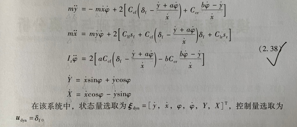
Equation (2.38) is a nonlinear dynamic equation considering lateral and longitudinal tire slip, which is established by assuming that the front wheel deflection δf is small and the tire model operates in the linear region.
The trajectory tracking belongs to the transverse control, and the control quantity is the front wheel angle δf. Here, the default longitudinal velocity Vx is constant, and the purpose of the trajectory tracking is to make the vehicle’s traverse angle φ and transverse position Y close to the φ_ref and Y_ref of the reference trajectory.
The state quantities ξ = [ y_dot, x_dot, φ, φ_dot, Y, X ] and the output quantities η = [ φ ; Y ] are chosen, and a nonlinear model is obtained:

1.1.2 Linear time-varying prediction model derivation
1. Discretization: the nonlinear equation (2.29) is discretized at k moments using the forward Euler method
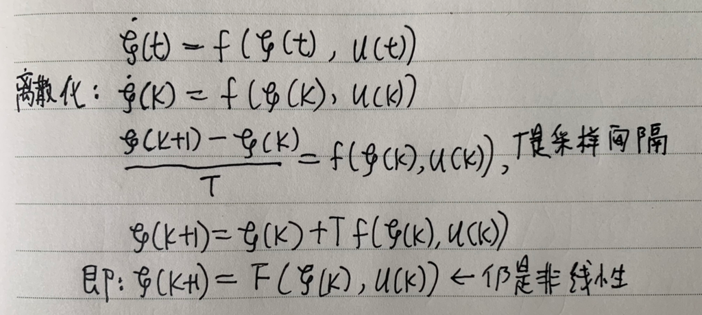
2. Linearization
The linearization method Taylor Expansion first requires the selection of a starting reference point, which can be chosen from the reference system method, and the linearization method for state trajectories (refer to section 3.3.2 of the first edition of the textbook, this part of the second edition of the textbook is missing).
a. The reference system approach means that the reference control quantity, Uref , and the state quantity, ξref , are obtained in advance for each moment in time. b. The reference system approach means that the reference control quantity, Uref , and the state quantity, ξref . i.e., it has been fully passed on the desired trajectory. This is designed to eliminate the deviation between the current vehicle state and the state of the reference system, and is essentially not a direct deviation comparison with the desired path, but a comparison with the reference value. The disadvantage of this approach is that a reference system needs to be acquired in advance. The desired trajectories in this chapter are only X_predict, Y_ref and φ_ref, which do not contain all the states, so it is not possible to obtain a set of reference systems in advance, so the state trajectory method is used.
b. State trajectory method: At the working point at time t, a constant control quantity ut is applied to the system to obtain a state trajectory ξt, which is linearized at the time t. The state trajectory is then linearized to the state trajectory ξt, which is then linearized to the state trajectory ξt.
difficultyThe so-called constant control quantity ut is the constant quantity u(k-1) used later, which is applied to the system before the trajectory tracking control, and this initial control quantity will be applied to the system constantly throughout the trajectory tracking process, and will not disappear with the changes of the system state and the control quantity, and the optimal Δu(k) obtained by each solution is only an increment compensated on the basis of the u(k-1) of the previous moment. The optimal Δu(k) obtained from each solution is only an increment compensated on the basis of u(k-1) of the previous moment, and this increment has no effect on the ut originally applied to the system, i.e., u(k-1), which is commonly understood as u(k+Np)=u(k-1) + Δu(k) + Δu(k+2) + … + Δu(k+Np). + Δu(k+Np-1) + Δu(k+Np), i.e., the change in the gain of the control quantity by Δu(k) obtained from each solution is superimposed on the next moment.
difficulty2: Here u(k-1) is actually the amount of control that has already been applied to the vehicle when no control increment has been applied, which means that it is the embodiment of the amount of control of the previous moment in the current moment, because no control increment has been applied yet, so it can naturally represent the amount of control of the previous moment.
The Taylor expansion is first performed at the working point (ξ0,u0) at time t=0, ignoring higher order terms:
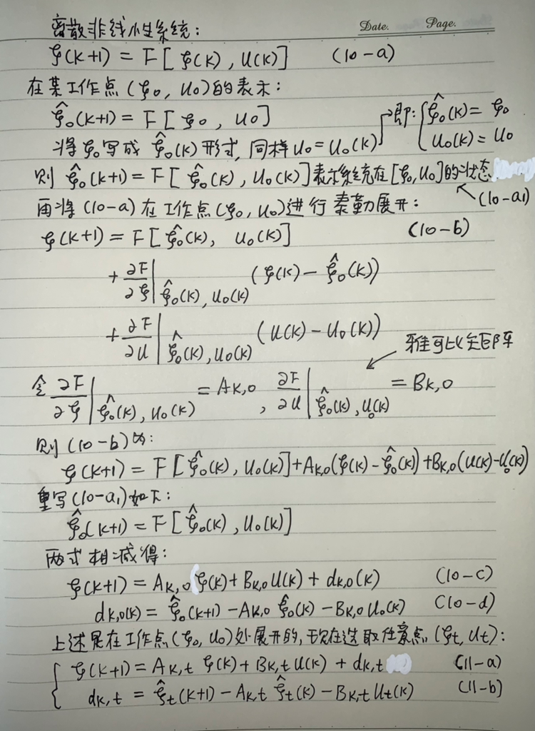
(The (11-a) ξ(k + 1) expression is the linear time-varying prediction model. Ak,t , Bk,t and dk,t indicate that this is a time-varying system LTV, which requires the coefficients to be solved online. The disadvantage of this model is that the expression does not contain the increment of the control quantity Δu(k), which prevents it from being constrained by ΔUmin and ΔUmax, and if the steering wheel is turned too much during driving, it will give a bad experience to the occupants of the car, so it is now necessary to construct a new form in order to contain the constraints on Δu(k):
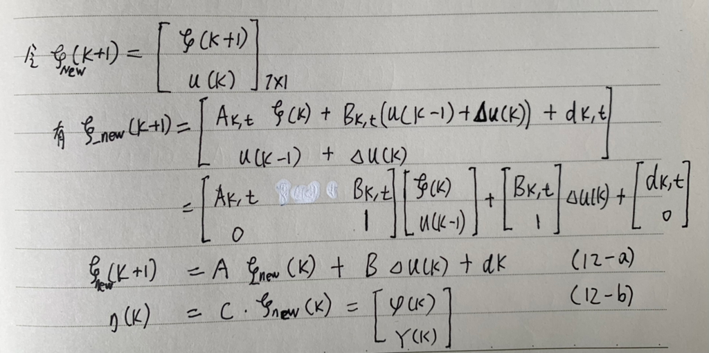
1.2 Model Predictive Controller Design
With the constraints on Δu(k) in place, the design of the MPC can begin, starting with the design of the objective function.
1.2.1 Objective function design
Given the higher complexity of the vehicle dynamics model and more constraints, it is very likely that the controller will fail to find an optimal solution within the specified time during execution, when the vehicle steering wheel is in a dangerous state of loss of control. To circumvent this situation, a relaxation factor ρ is added to the objective function.
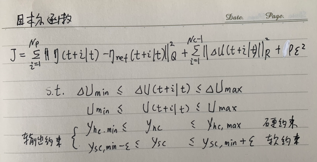
Note that here a larger ρ means that the conditions for the solution are more relaxed, but too large a ρ also means that the tracking is not as good as it could be.
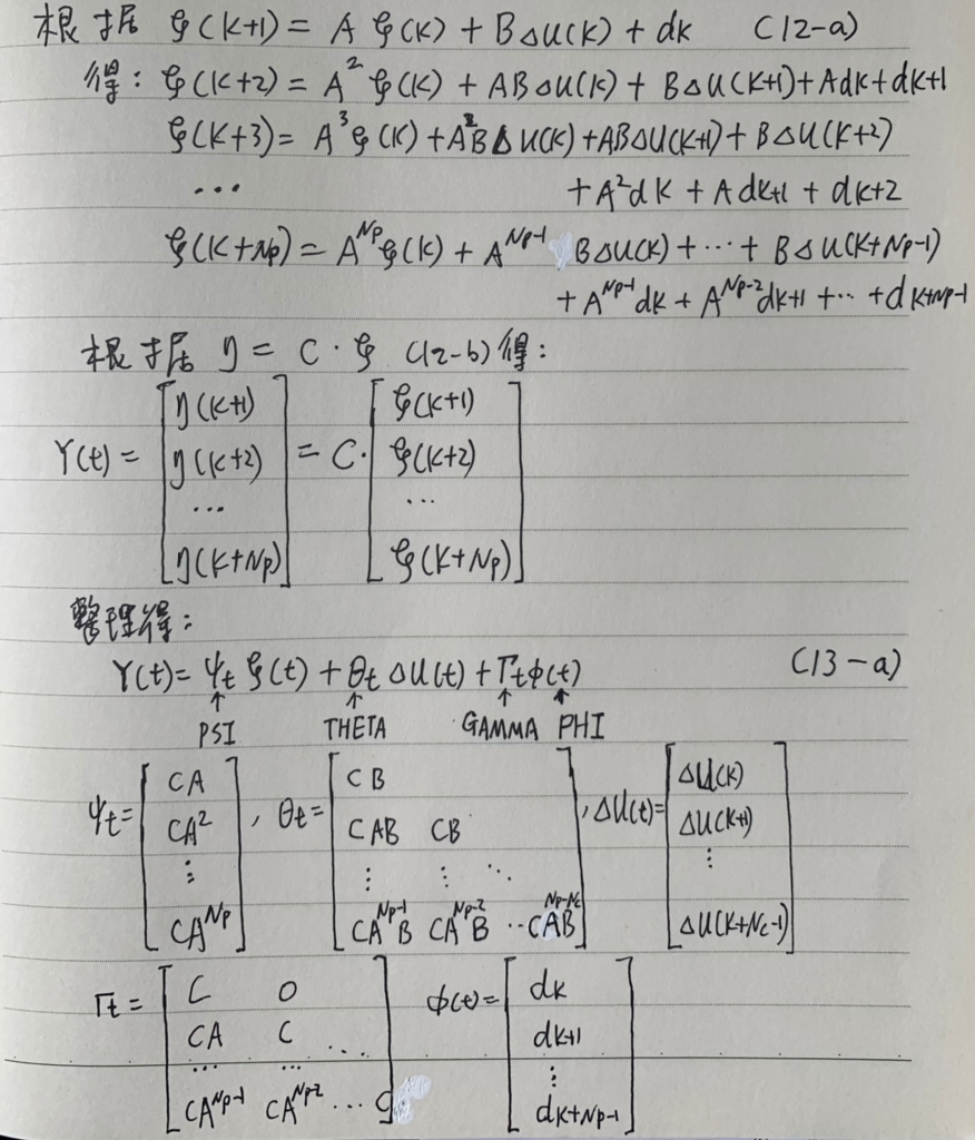
The Y(t) expression of Eq. (13-a) contains ξ(k+i) in the future Np prediction time domains by substituting Y(t) into the objective function.
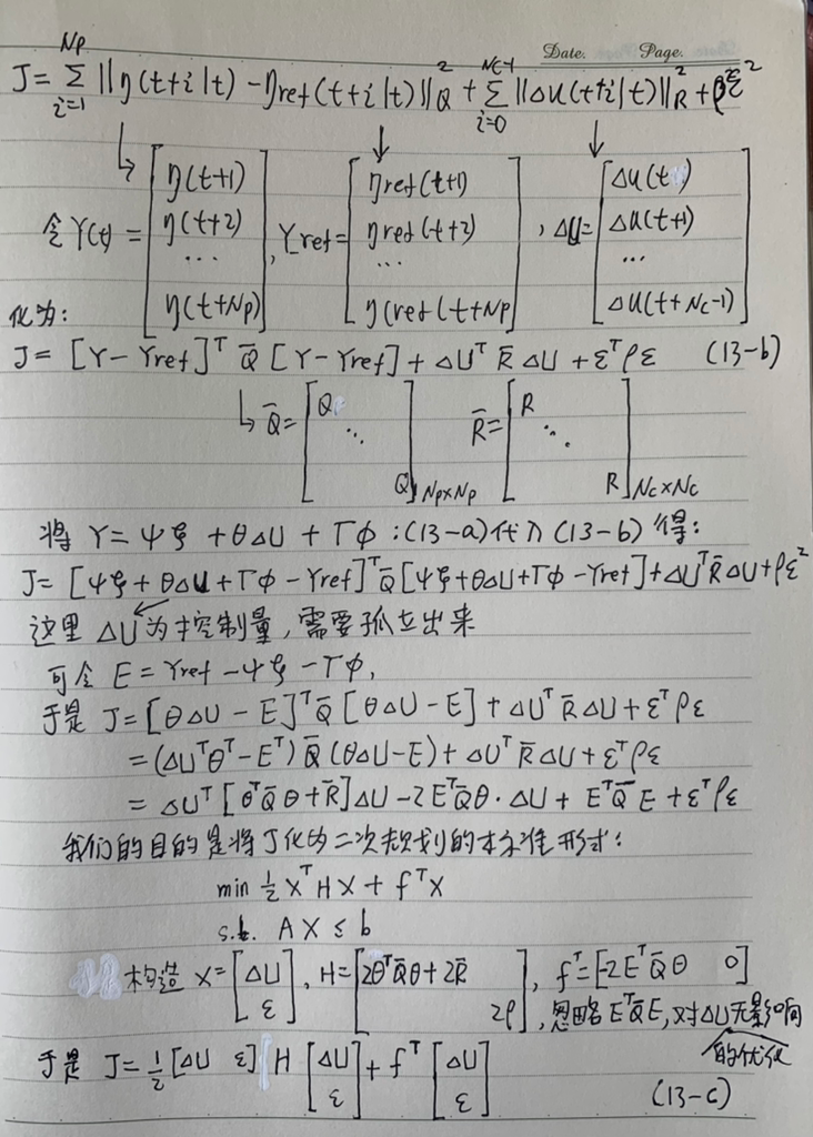
Equation (13-c) is a standard form of quadratic programming, where the solution X to be solved has been augmented from a one-dimensional Δδf to a two-dimensional augmented matrix containing ε. The design of the constraints follows.
1.2.2 Binding design
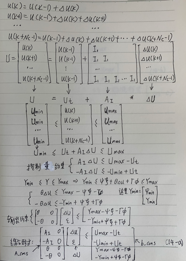
The control quantity u(k) constraint and the constraints of output quantities φ(k) and Y(k):
controls the constraints on the increment Δu:
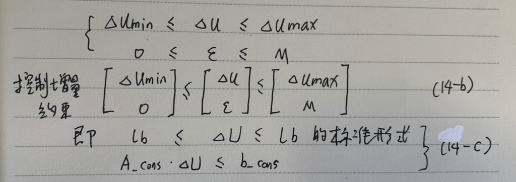
Equation (14-a) is the combined form that combines the control and output quantities, and Equation (14-b) is the constraints on the control increments and relaxation factors. The linear time-varying prediction model for trajectory tracking has been completed so far, and the next work is to analyze the code in conjunction with a joint simulation with carsim to see the effect of trajectory tracking.
2 Code Parsing
2.1 Template framework
2.1.1 S-Function
function [sys,x0,str,ts] = chapter5_2_2(t,x,u,flag) % u denotes input from carsim
switch flag,
 case 0
  [sys,x0,str,ts] = mdlInitializeSizes; % Initialize some basic dimensions of the system parameters
 case 2
  sys = mdlUpdates(t,x,u); % not used
 case 3
  sys = mdlOutputs(t,x,u); % the main module that implements the control algorithm
 case {1,4,9}
  sys = [];
 otherwise
  error(['unhandled flag = ',num2str(flag)]);
end
2.1.2 mdlInitializeSizes function
function [sys,x0,str,ts] = mdlInitializeSizes
sizes = simsizes;
sizes.NumContStates = 0; % The number of consecutive states is 0.
sizes.NumDiscStates = 6; % number of discrete states is 6
sizes.NumOutputs = 1; % number of outputs is 1, delta_f as output
sizes.NumInputs = 8; % The number of inputs is 8, from carsim, and includes 2 slip rates.
sizes.DirFeedthrough = 1; % The mdlOutputs function module is directly called with data from u, so it's 1
sizes.NumSampleTimes = 1;
sys = simsizes(sizes);
x0 = [0.001;0.0001;0.0001;0.00001;0.00001;0.00001]; % Initial values of the 6 state quantities
global U; % 1-dimensional control volume, front wheel angle output delta_f
U=[0]; % delta_f(0)=0, front wheel angle 0° at startup
str = [];
ts = [0.05 0]; % The simulation interval is 0.05 seconds, the second term is 0 to indicate that the simulation starts at 0 seconds immediately
2.1.3 mdlUpdates() function
function sys = mdlUpdates(t,x,u) % This part is not used.
sys = x;
2.1.4 mdlOutputs() function
u denotes the 8 state inputs from carsim.
function sys = mdlOutputs(t,x,u)
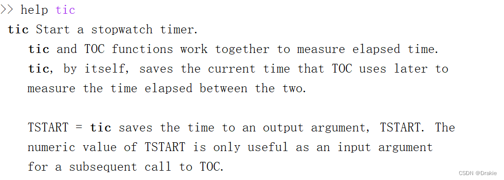
    tic % Start the clock
    fprintf('Update start, t=%6.3f\n',t) % Log the start of the control action at the current moment
    Nx=6;
    Nu=1;
    Ny=2;
    Np =20;
    Nc=5;
    T=0.05; % Sampling time
2.2 MPC Algorithm Body
tic meaning:
The following section is parameterized by the vehicle body in order to solve for the Jacobi matrices a and b
%% a b Constant parameter: vehicle body
    Sf=0.2; Sr=0.2;
    lf=1.232;lr=1.468;
    Ccf=66900;Ccr=62700;
    Clf=66900;Clr=62700;
    m=1723;g=9.8;I=4175;
%% a b Variable parameters, carsim real-time acquisition
    y_dot=u(1)/3.6; % Km/h => m/s
    x_dot=u(2)/3.6+0.0001; % Prevent the denominator from being 0
    phi=u(3)*3.141592654/180; % degree => rad
    phi_dot=u(4)*3.141592654/180;
    Y=u(5);
    X=u(6);
    Y_dot=u(7); % Longitudinal slip rate of front wheel
    X_dot=u(8); % Rear wheel longitudinal slip rate
    global U; % Control volume
    delta_f=U(1);
    fprintf('Update start, u(1)=%4.2f\n',U(1)) % The log records the amount of control per control cycle
Jacobi matrix a b Solve
Next comes the matrix expressions for the Jacobi matrices a and b. Only the results are written here:
%% a b
    global a b;
    a=[                 1 - (259200*T)/(1723*x_dot),                                                         -T*(phi_dot + (2*((460218*phi_dot)/5 - 62700*y_dot))/(1723*x_dot^2) - (133800*((154*phi_dot)/125 + y_dot))/(1723*x_dot^2)),                                    0,                     -T*(x_dot - 96228/(8615*x_dot)), 0, 0
        T*(phi_dot - (133800*delta_f)/(1723*x_dot)),                                                                                                                  (133800*T*delta_f*((154*phi_dot)/125 + y_dot))/(1723*x_dot^2) + 1,                                    0,           T*(y_dot - (824208*delta_f)/(8615*x_dot)), 0, 0
                                                  0,                                                                                                                                                                                  0,                                    1,                                                   T, 0, 0
            (33063689036759*T)/(7172595384320*x_dot), T*(((2321344006605451863*phi_dot)/8589934592000 - (6325188028897689*y_dot)/34359738368)/(4175*x_dot^2) + (5663914248162509*((154*phi_dot)/125 + y_dot))/(143451907686400*x_dot^2)),                                   0, 1 - (813165919007900927*T)/(7172595384320000*x_dot), 0, 0
                                          T*cos(phi),                                                                                                                                                                         T*sin(phi),  T*(x_dot*cos(phi) - y_dot*sin(phi)),                                                   0, 1, 0
                                         -T*sin(phi),                                                                                                                                                                         T*cos(phi), -T*(y_dot*cos(phi) + x_dot*sin(phi)),                                                   0, 0, 1];


    b=[                                                               133800*T/1723
       T*((267600*delta_f)/1723 - (133800*((154*phi_dot)/125 + y_dot))/(1723*x_dot))
                                                                                 0
                                                5663914248162509*T/143451907686400
                                                                                 0
                                                                                 0];
The purpose of defining the Jacobi matrices a and b is to solve for the A and B matrices:
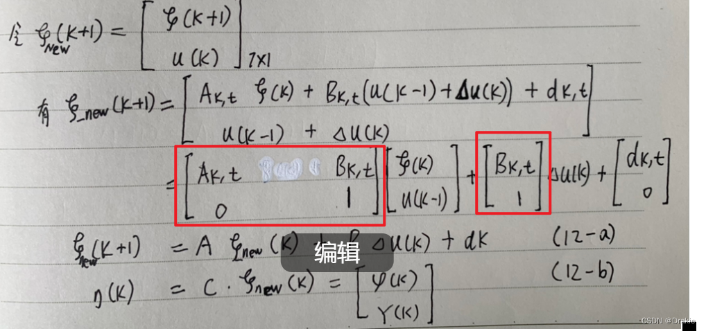
Code Implementation:
    %%  A B C
    A_cell=cell(2,2);
    A_cell{1,1}=a;
    A_cell{1,2}=b;
    A_cell{2,1}=zeros(Nu,Nx);
    A_cell{2,2}=eye(Nu);
    A=cell2mat(A_cell);

    B_cell=cell(2,1);
    B_cell{1,1}=b;
    B_cell{2,1}=eye(Nu);
    B=cell2mat(B_cell);

    C=[0 0 1 0 0 0 0;
       0 0 0 0 1 0 0;];
The purpose of the A and B matrices obtained here is to obtain the ψ θ Γ Φ matrices, cf. Eq. (13-a):
![]()
Since θ is called by the matrix E H f at the same time, θ can be realized here first:
%% THETA (called by E H f)
    THETA_cell=cell(Np,Nc);
    for j=1:1:Np
        for k=1:1:Nc
            if k<=j
                THETA_cell{j,k}=C*A^(j-k)*B;
            else
                THETA_cell{j,k}=zeros(Ny,Nu);
            end
        end
    end
    THETA=cell2mat(THETA_cell);
Our ultimate goal is to define E H f matrices in order to construct quadratic programming standard type matrices. Below we implement the E H and f matrices sequentially, combining the formulas to define the matrices sequentially makes the code segment more intuitive.
E Matrix
![]()
The first item is the reference track, which can be generated from an external file or defined directly.
Reference trajectory Y ref
%% Y_ref
    % phi_ref Y-ref
    shape=2.4;%parameter name for reference trajectory generation
    dx1=25;dx2=21.95;% doesn't have any real meaning, it's just the name of the parameter
    dy1=4.05;dy2=5.7;% doesn't have any real meaning, it's just the name of the parameter
    Xs1=27.19;Xs2=56.46;% parameter name, the above parameters are to generate our double shift line
    X_predict= zeros(Np,1);% used to hold the longitudinal position information in the predicted time domain, which is the basis for computing the desired trajectory
    phi_ref = zeros(Np,1);% used to save the reference transverse pendulum angle information in the prediction time domain
    Y_ref = zeros(Np,1);% used to hold the reference lateral position information in the prediction time domain
    % Yita_ref
    Yita_ref_cell=cell(Np,1); % =========== Here the naming should be Y_out_ref_cell because the dimension of η is 2, not Np, but because of the naming conflict between the output quantity Y and the horizontal coordinates ================
    T_all=20; % Total simulation time to prevent the computation of the desired trajectory from going out of bounds
    for p=1 Np % exceeding the simulation duration.
        if t+p*T>T_all
            X_DOT=x_dot*cos(phi)-y_dot*sin(phi);
            X_predict(Np,1)=X+X_DOT*Np*T;
            z1=shape/dx1*(X_predict(Np,1)-Xs1)-shape/2;
            z2=shape/dx2*(X_predict(Np,1)-Xs2)-shape/2;
            Y_ref(p,1)=dy1/2*(1+tanh(z1))-dy2/2*(1+tanh(z2));
            phi_ref(p,1)=atan(dy1*(1/cosh(z1))^2*(1.2/dx1)-dy2*(1/cosh(z2))^2*(1.2/dx2));
            Yita_ref_cell{p,1}=[phi_ref(p,1);Y_ref(p,1)];
        else % Within the simulation time (normal execution part)
            X_DOT = x_dot*cos(phi) - y_dot*sin(phi); % Slope of X, given by nonlinear dynamics equation (2.29)
            X_predict(p,1)=X+X_DOT*p*T; % X is the current longitudinal coordinate of the vehicle output by carsim, and X_predict(p,1) represents the longitudinal coordinate of the next moment
            z1=shape/dx1*(X_predict(p,1)-Xs1)-shape/2;
            z2=shape/dx2*(X_predict(p,1)-Xs2)-shape/2;
            Y_ref(p,1)=dy1/2*(1+tanh(z1))-dy2/2*(1+tanh(z2)); % Cross reference for next moment
            phi_ref(p,1)=atan(dy1*(1/cosh(z1))^2*(1.2/dx1) - dy2*(1/cosh(z2))^2*(1.2/dx2)); % Transverse Pendulum Angle Reference for next moment
            Yita_ref_cell{p,1}=[phi_ref(p,1);Y_ref(p,1)]; % [phi_rel; Y_ref]
        end
    end
    Yita_ref=cell2mat(Yita_ref_cell); % Y_ref matrix normalization
Next realize that ψ
    %% ψ  PSI
    PSI_cell=cell(Np,1);
    for j=1:1:Np
        PSI_cell{j,1}=C*A^j;
    end
    PSI=cell2mat(PSI_cell);
and then ξ, where ξ is the augmented generalized matrix after reconstruction:

    %% ξ  kesi
    kesi=zeros(Nx+Nu,1); % ξnew(k)=[ξ(k); u(k-1)]
    kesi(1)=y_dot;
    kesi(2)=x_dot;
    kesi(3)=phi;
    kesi(4)=phi_dot;
    kesi(5)=Y;
    kesi(6)=X;
    kesi(7)=U(1); % u(k-1)
GAMMA
%% Γ  GAMMA
    GAMMA_cell=cell(Np,Np); % Dimension 20*20
    for p=1:1:Np;
        for q=1:1:Np;
            if q<=p; % lower triangular matrix
                GAMMA_cell{p,q}=C*A^(p-q);
            else
                GAMMA_cell{p,q}=zeros(Ny,Nx+Nu);
            end
        end
    end
    GAMMA=cell2mat(GAMMA_cell);
Finally, the implementation of Φ is a bit more complicated, first looking at the expression that
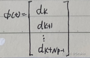
dk,t expression:
![]()
ξt_hat(k+1): here it needs to be understood:
%% φ   PHI
    % ξt_hat_(k+1) Prepare for solving PHI
    state_k1=zeros(Nx,1);% below starts equation (10-a1) i.e. value at moment k+1 = initial value at moment k + T * slope at moment k (equation 2.38)
    state_k1(1,1)=y_dot+T*(-x_dot*phi_dot+2*(Ccf*(delta_f-(y_dot+lf*phi_dot)/x_dot)+Ccr*(lr*phi_dot-y_dot)/x_dot)/m);
    state_k1(2,1)=x_dot+T*(y_dot*phi_dot+2*(Clf*Sf+Clr*Sr+Ccf*delta_f*(delta_f-(y_dot+phi_dot*lf)/x_dot))/m);
    state_k1(3,1)=phi+T*phi_dot;
    state_k1(4,1)=phi_dot+T*((2*lf*Ccf*(delta_f-(y_dot+lf*phi_dot)/x_dot)-2*lr*Ccr*(lr*phi_dot-y_dot)/x_dot)/I);
    state_k1(5,1)=Y+T*(x_dot*sin(phi)+y_dot*cos(phi));
    state_k1(6,1)=X+T*(x_dot*cos(phi)-y_dot*sin(phi));
Since the Jacobi matrices a and b have been defined earlier, it is now straightforward to write the dk,t matrix form:
![]()
% dk in preparation for solving PHI
    d_k=zeros(Nx,1); % (6,1)
    d_k=state_k1-a*kesi(1:6,1)-b*kesi(7,1); % Equation (11-b) d_k=ξt_hat_(k+1)-Ak,t * ξt_hat_(k) -Bk,t * u(k-1)
Here you also need to refactor d_piao_k:

% d_piao_k Prepare for solving PHI
    d_piao_k=zeros(Nx+Nu,1) % (7,1)
    d_piao_k(1:6,1)=d_k; % d_piao_k=[dk; 0], see equation (12-a)
    d_piao_k(7,1)=0;
Eventually the Φ matrix can be solved:
% PHI final solution
    PHI_cell=cell(Np,1); % φ(20*7,1)
    for p=1:1:Np;
        PHI_cell{p,1}=d_piao_k;
    end
    PHI=cell2mat(PHI_cell);
The E-matrix can be realized next
![]()
%% E Final Solution
    E=zeros(Ny*Np,1);% source code named error_1
    E=Yita_ref-PSI*kesi-GAMMA*PHI; % E=Yref-phi*ξ-Γφ,here Yita_ref is Yref
H matrix
% Q
    Q_cell=cell(Np,Np);
    for i=1:1:Np;
        for j=1:1:Np;
            if i==j
                Q_cell{i,j}=[2000 0;0 10000;]; % Transverse hem angle weights, lateral position weights respectively
            else
                Q_cell{i,j}=zeros(Ny,Ny); % Ny = 2
            end
        end
    end
    Q=cell2mat(Q_cell);
% R
    R=5*10^5*eye(Nu*Nc);
% Relaxation factor ρ
    Row=1000;
 % H Final Solution
    H_cell=cell(2,2);
    H_cell{1,1}=THETA'*Q*THETA+R; % H = θ'* Q * θ + R
    H_cell{1,2}=zeros(Nu*Nc,1);
    H_cell{2,1}=zeros(1,Nu*Nc);
    H_cell{2,2}=Row;
    H=cell2mat(H_cell);
    H=(H+H')/2; % Ensure that the H-matrix is a strictly symmetric array
f Matrix
    f_cell=cell(1,2);
    f_cell{1,1}=2 * E' * Q * THETA;
    f_cell{1,2}=0;
    f=-cell2mat(f_cell);
So far the full element matrix H f has been realized, and the next two can start defining the constraint matrix.
constraint matrix (math.)
%% constraints on the control quantity u(k).
    A_t=zeros(Nc,Nc);
    for p=1:1:Nc
        for q=1:1:Nc
            if q<=p
                A_t(p,q)=1;
            else
                A_t(p,q)=0;
            end
        end
    end
    A_I=kron(A_t,eye(Nu)); % Here A_I is A_t because Nu=1
    Ut=kron(ones(Nc,1),U(1)); Ut = u(k -1)
    umin=-0.1744; % Upper constraint on the front wheel deflection angle
    umax=0.1744; % Lower constraint on the front wheel deflection angle
    Umin=kron(ones(Nc,1),umin);
    Umax=kron(ones(Nc,1),umax);
The constrained form of the output quantity Y(k):
%% Output constraints
    ycmax=[0.21; 5]; % Constraints on transverse pendulum angle and longitudinal position
    ycmin=[-0.3;-3];
    Ycmax=kron(ones(Np,1),ycmax);
    Ycmin=kron(ones(Np,1),ycmin);
An augmented and generalized hybrid form of the u(k) and Y(k) constraints:
% Combining control volume constraints and output volume constraints
    A_cons_cell={A_I zeros(Nu*Nc,1);-A_I zeros(Nu*Nc,1);THETA zeros(Ny*Np,1);-THETA zeros(Ny*Np,1)};
    b_cons_cell={Umax-Ut;-Umin+Ut;Ycmax-PSI*kesi-GAMMA*PHI;-Ycmin+PSI*kesi+GAMMA*PHI};
    A_cons=cell2mat(A_cons_cell);%(Solve equation) state quantity inequality constrained gain matrix, converted to range of absolute values
    b_cons=cell2mat(b_cons_cell);%(Solve the equation) the value of the state quantity inequality constraints
The constraints on Δu(k), which are the constraints on the standard state quantities X of the QP solution equations:
%% Control increment constraints
    delta_umin=-0.0148*0.4; % Lower constraint on the amount of change in the front wheel deflection angle
    delta_umax= 0.0148*0.4; % Upper constraint on the amount of change in front wheel declination
    delta_Umin=kron(ones(Nc,1),delta_umin);
    delta_Umax=kron(ones(Nc,1),delta_umax);
    M=10; % Upper bound on ε
    lb=[delta_Umin;0]; % Augmented lower bound constraint on [Δu(k);ε] lb
    ub=[delta_Umax;M]; % Augmented upper bound constraint on [Δu(k);ε] ub
quadprog solver
Call quadprog, matlab‘s own quadratic programming solver, which is the core of the solver.
%% quadprog solver
options = optimset('Algorithm','interior-point-convex'); The internal point method is used to solve %
x_start=zeros(Nc+1,1); % initial value of [Δu(k);ε] is 0
[X,fval,exitflag]=quadprog(H,f,A_cons,b_cons,[],[],lb,ub,x_start,options);
The solution of % [Δu(k);ε] is stored in the variable X and contains Δu(k+i) for the next Nc time points
Result processing, output the result of the calculation u(k) to carsim:
%% Calculated output
u_piao=X(1); % Extract the Δu(k) of the first moment from the Δu(k+i) of the Nc future moments as the optimal solution of the current moment
U(1)=kesi(7,1)+u_piao; % here kesi(7,1) is u(k-1), plus Δu(k), is the actual output u(k) at the current moment.
sys= U; % Here U is used as the output of simulink and copied directly to carsim for front wheel angle control
toc % One full control cycle timed out
Now that the full matlab code has been implemented, co-simulation will be performed in the next section.
3. carsim, simulink co-simulation
This section mainly explains the validation of the designed MPC controller by building simulink/carsim co-simulation platform with an example. The following figure shows an example of the joint simulation of carsim and simulink for the MPC trajectory tracking controller based on the dynamics model. carsim version is 8.02, matlab version is 2018a。
3.1 Carsim setup
Including vehicle parameter setting, simulation working condition setting, input/output interface setting, and simulation result viewing.
3.1.1 Vehicle parameterization


The next step is the specific setting of vehicle parameters, including vehicle size information and tire information.


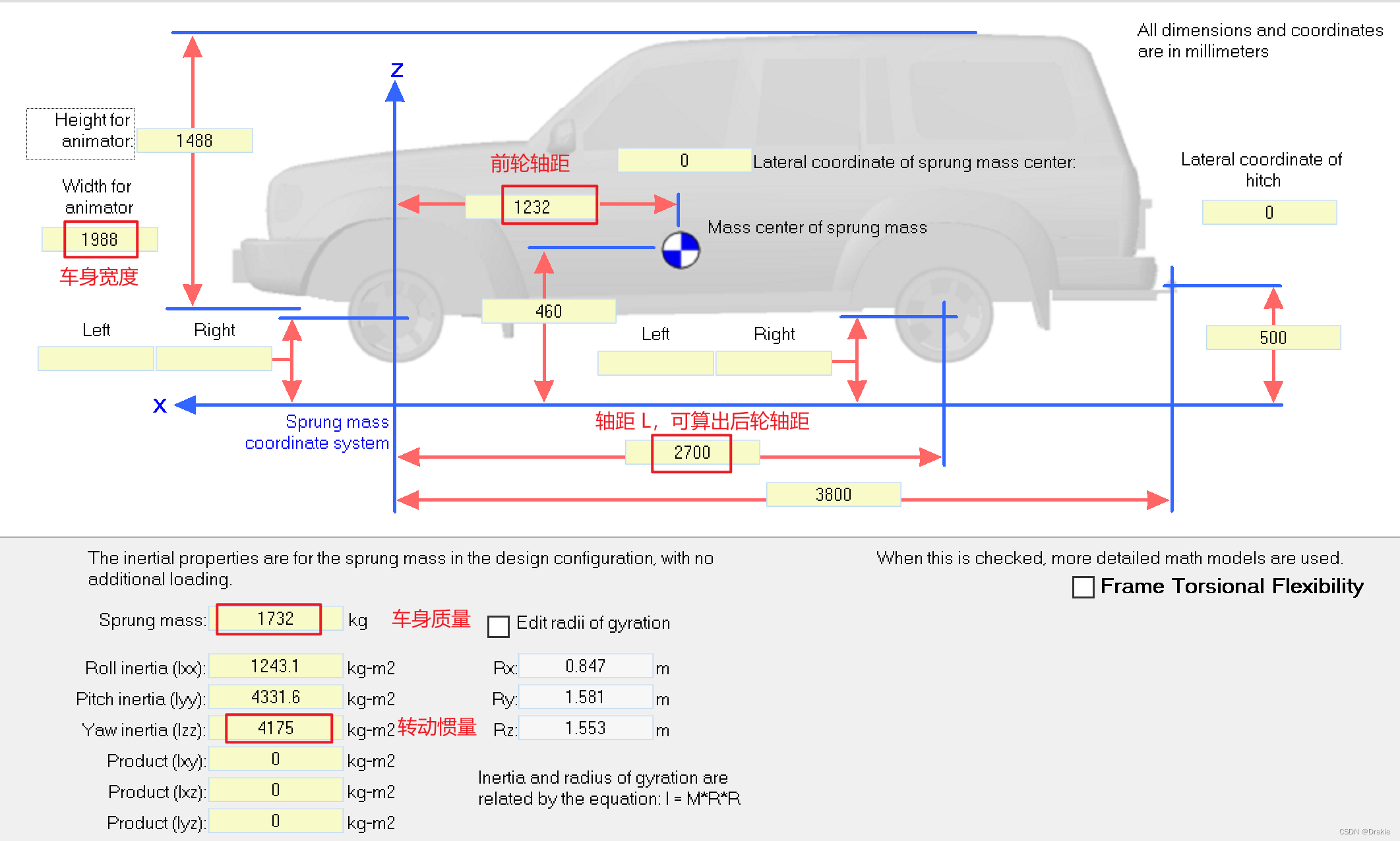
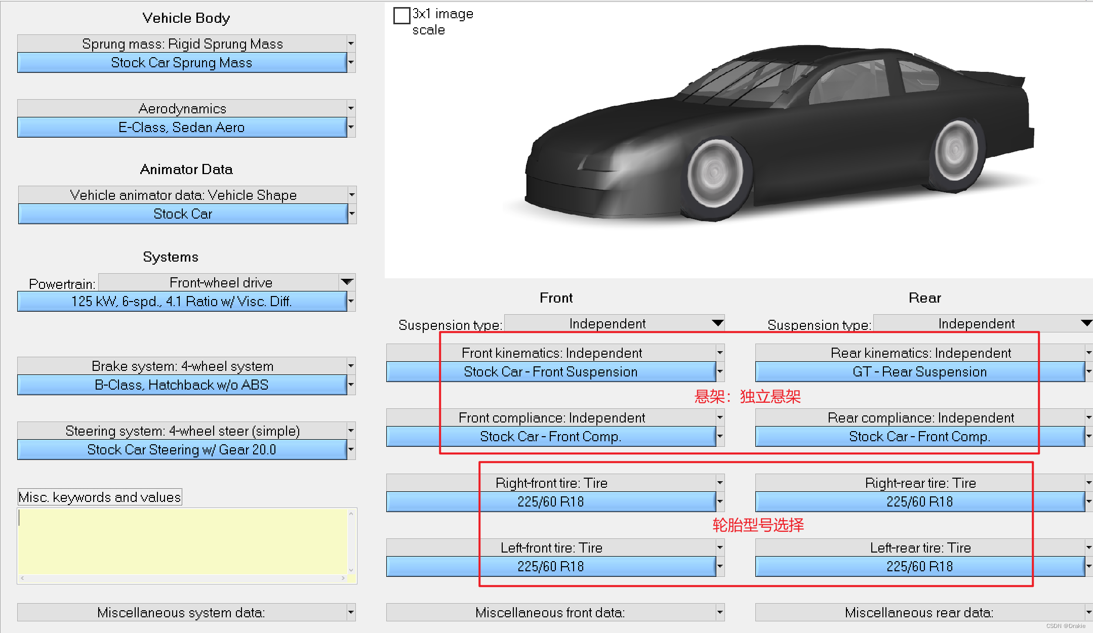
Return to the Vehicle Parameter Setting screen and select the suspension and tire model.
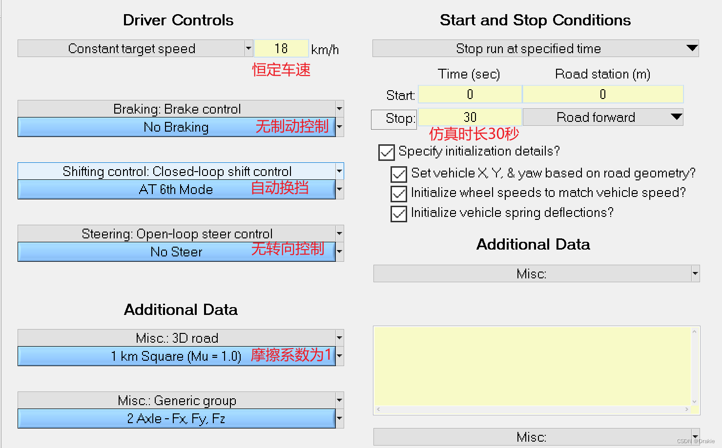
3.1.2 Simulation working condition setting


3.1.3 Input and output settings
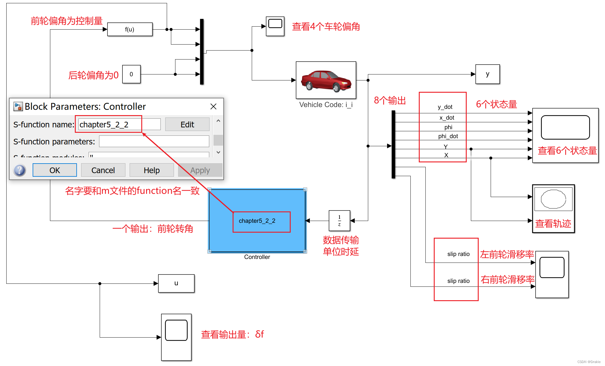
Since the trajectory following in this chapter is lateral control and only the front wheel corners are controlled, the input port of carsim selects the corners of the four tires of the vehicle. The angles of the 2 front wheels are provided by the controller and the angles of the 2 rear wheels are fixed at 0.0°. The output ports include 6 state quantities of the dynamical system and the slip rates of the 2 front wheels, for a total of 8 outputs.
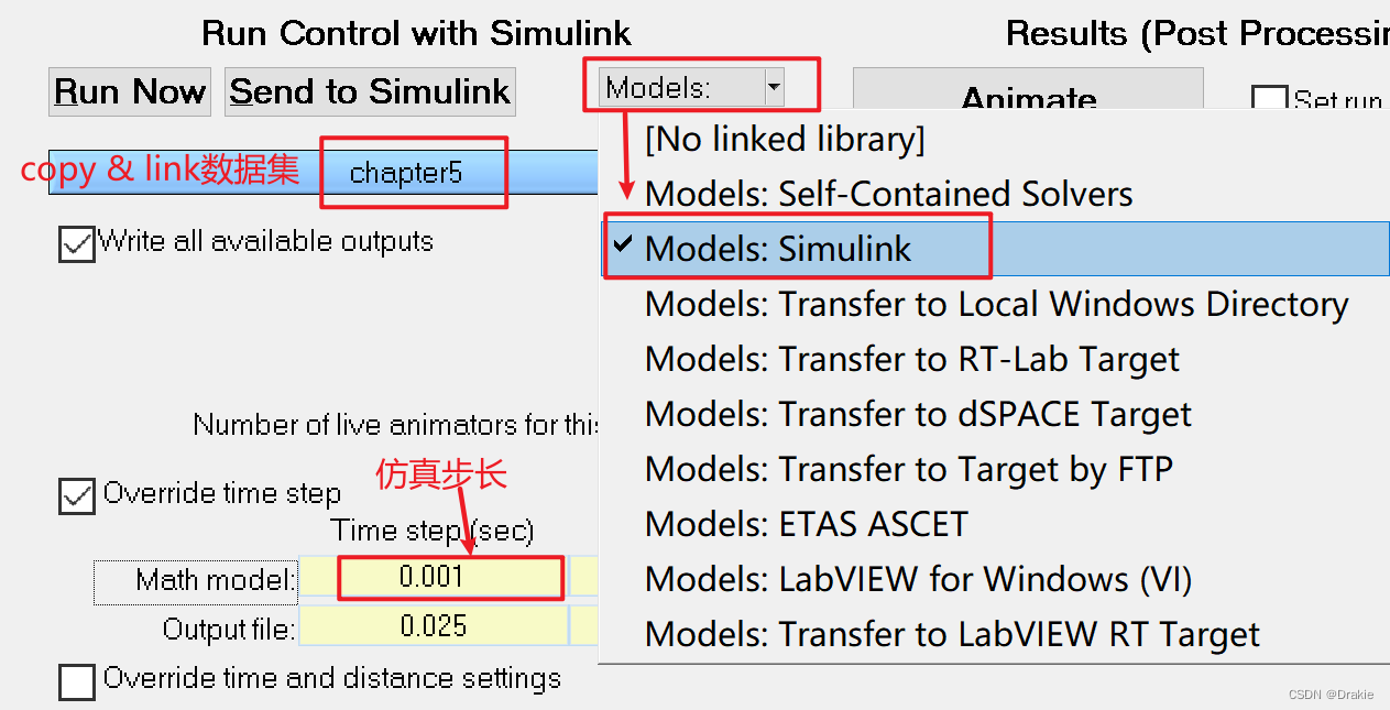
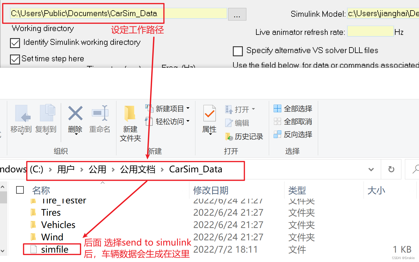



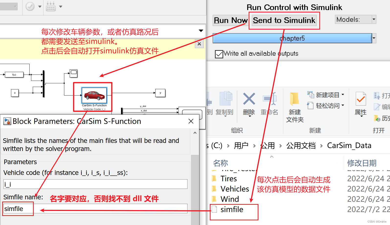
The data streaming between carsim and simulink as shown in the figure below is realized:

3.1.4 Simulation results: graphical curves
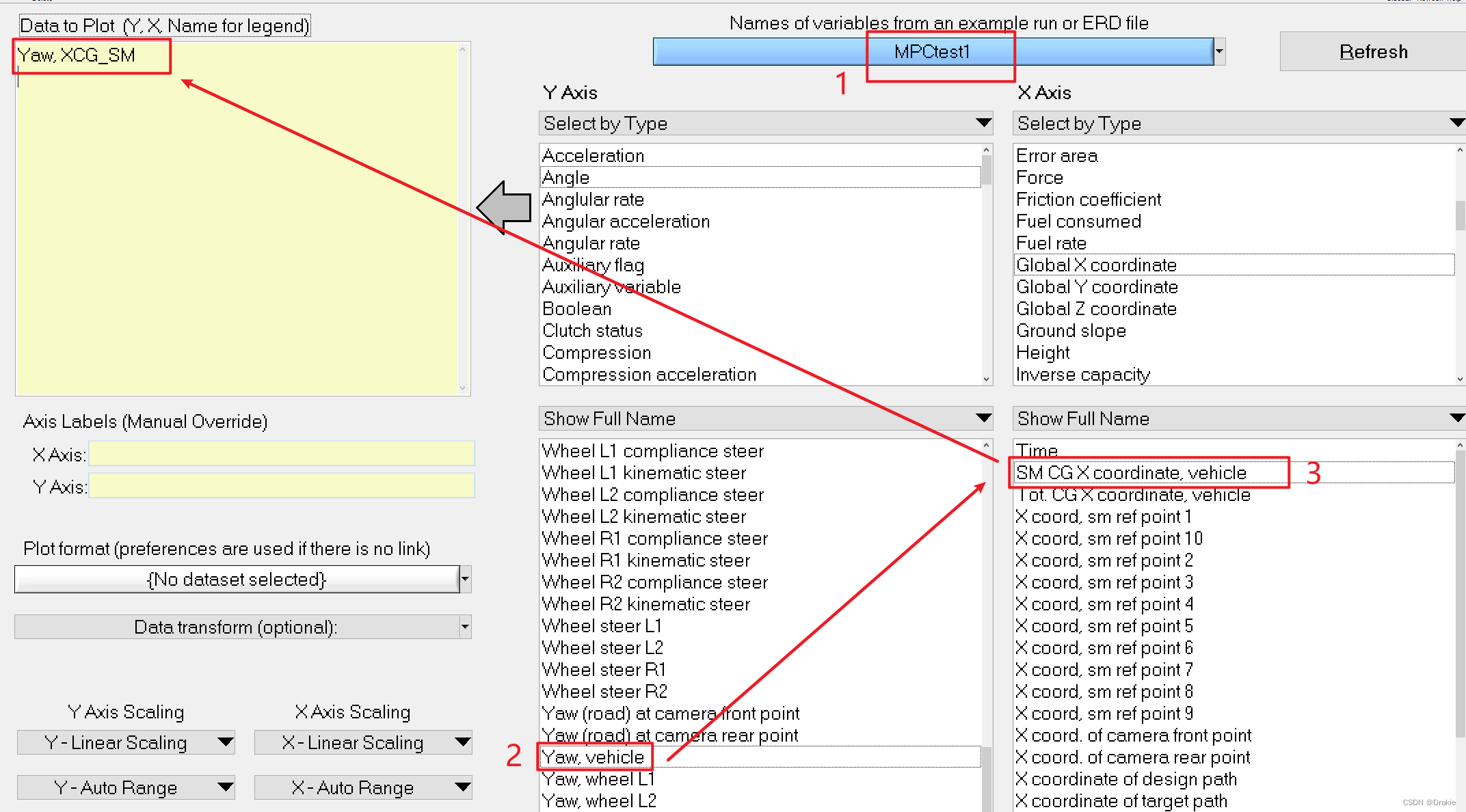
New dataset:

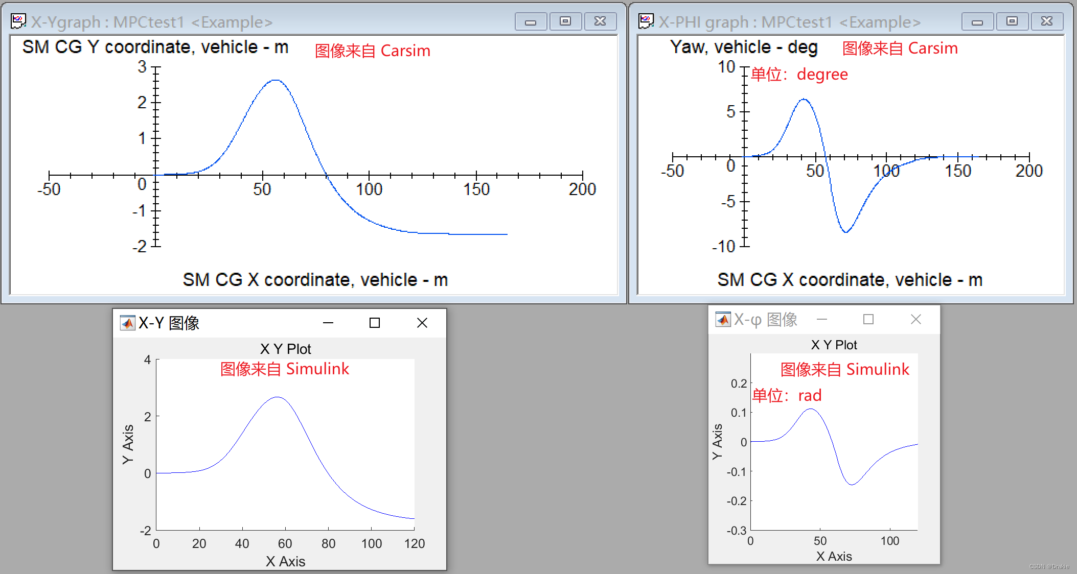
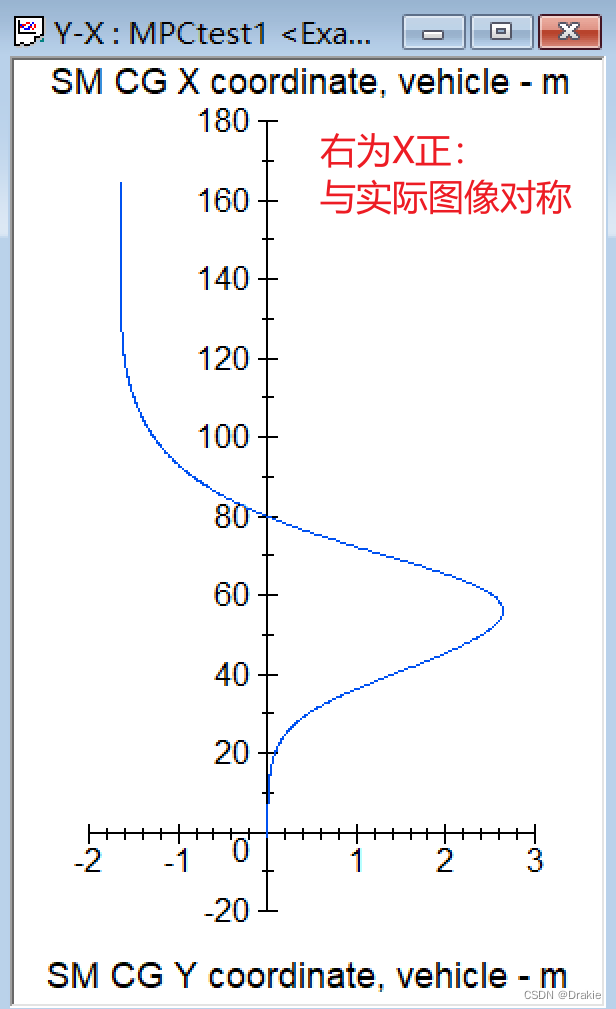
Add an image of the lateral position Y about X of the center of mass of the vehicle:
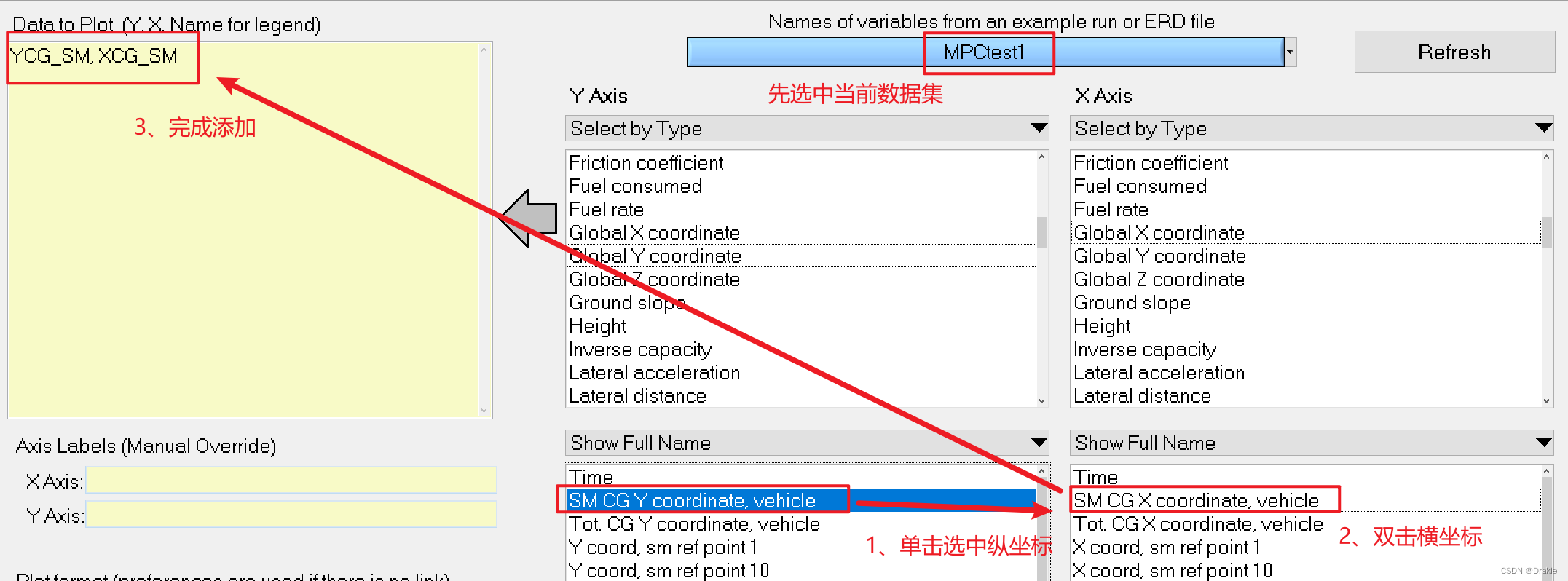
Add an image of the swing angle φ with respect to the longitudinal position X:
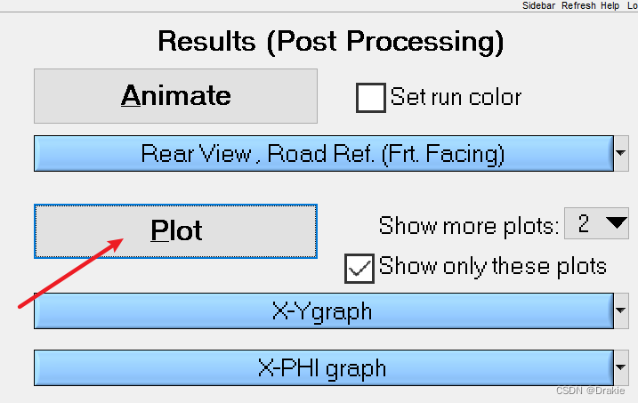
Click Plot to start drawing
The carsim graphical curves are compared with the data collected by simulink and the results are identical:
3.1.5 Simulation results: animation effects
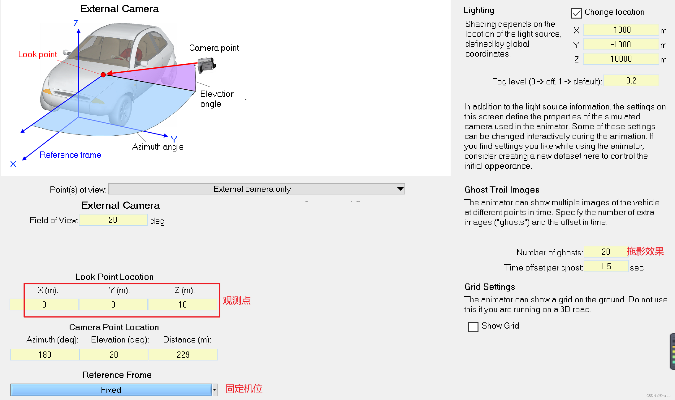
Go back to the main screen and select Perspective from the drop-down list, or New Custom Dataset:

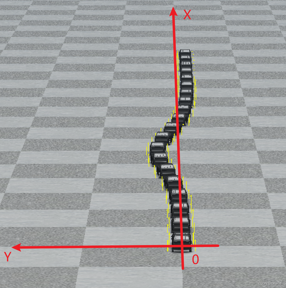
Enter the viewpoint setting interface, in order to show the tracking effect of the double-shift line, here choose the drag effect, i.e. Ghost Trail Images, select the number of drags, time interval, and set the observation viewpoint to a fixed viewpoint behind the starting point of the car body:
The tracking animation effect is as follows, and the actual double shift line motion trajectory of the vehicle can be observed:
3.2 simulink Simulation
3.2.1 carsim path addition
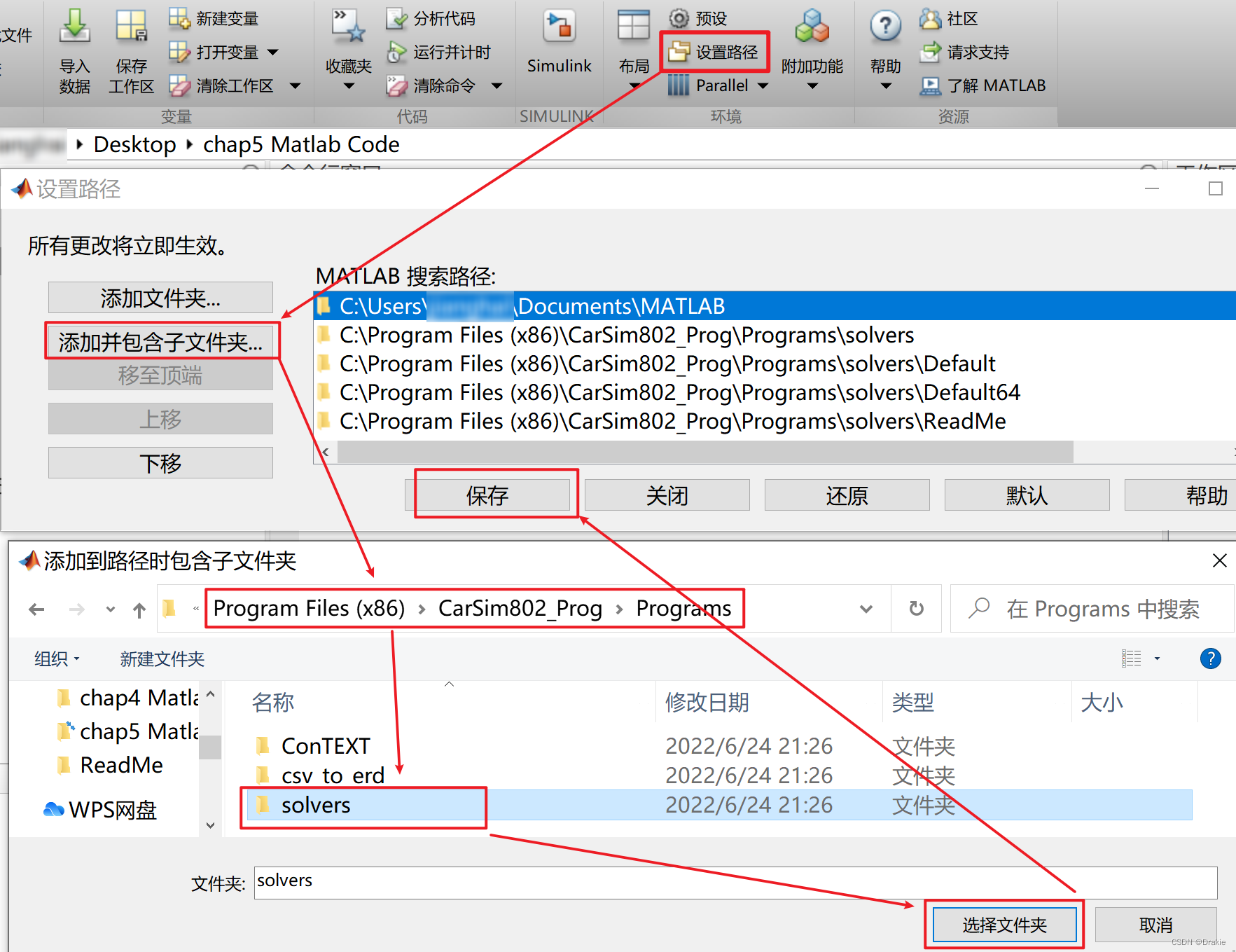
The Carsim module can be found in the Simulink Library Brower for MATLAB after restarting the computer.
3.2.2 Building Simulink
First make sure that matlab has the Autopilot Toolkit installed.

Some matlab versions can’t be displayed directly, so here’s the Fix.
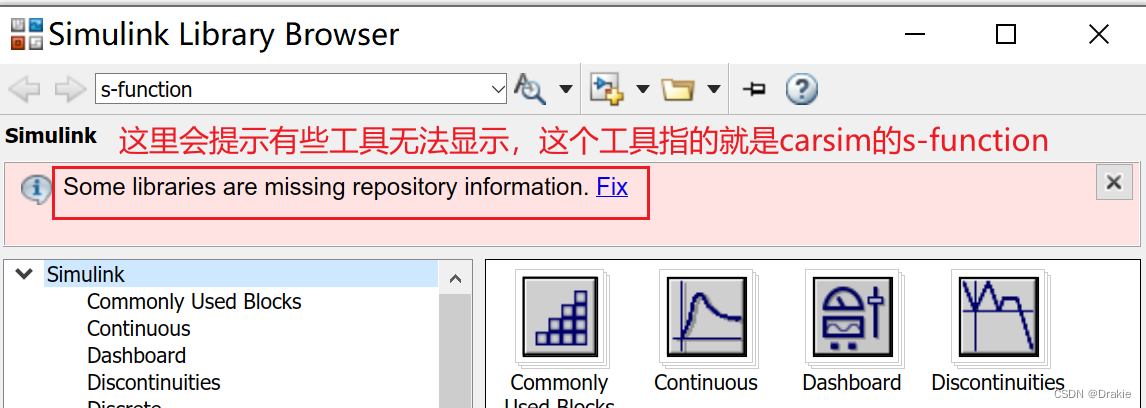
And then pick the second one.
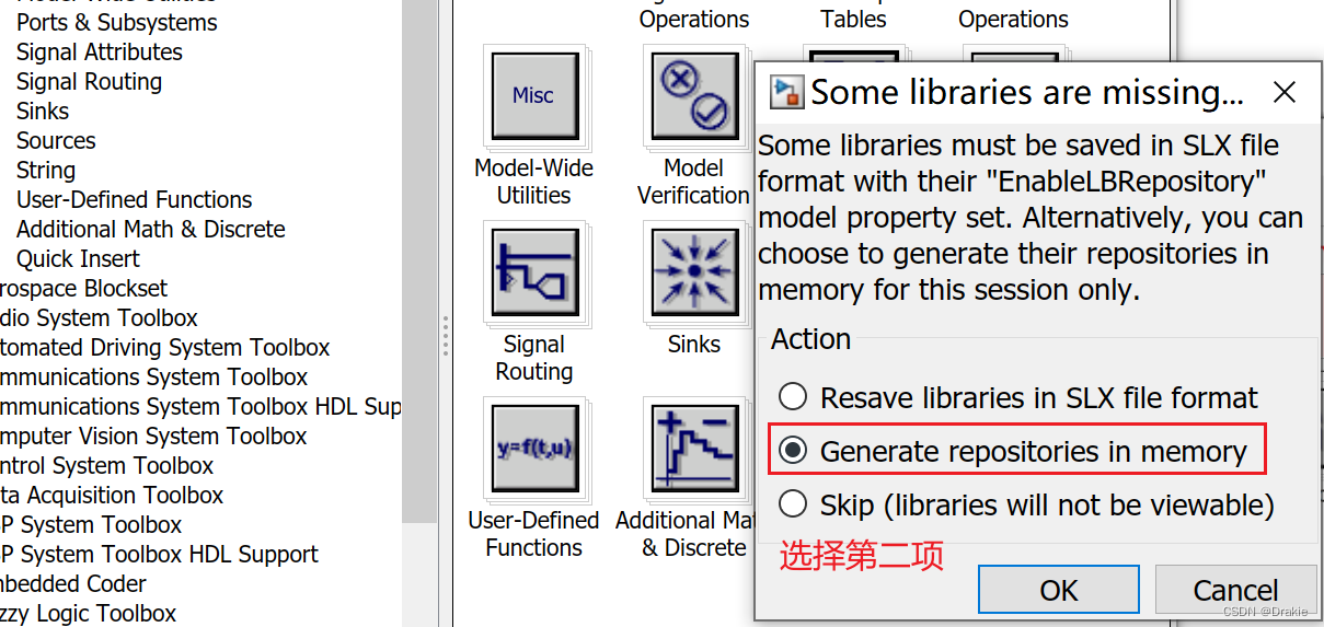
This is where you add the carsim s-function module

Here’s the complete simulink module that was built
Editing m-files in s-function

3.2.3 Simulation results
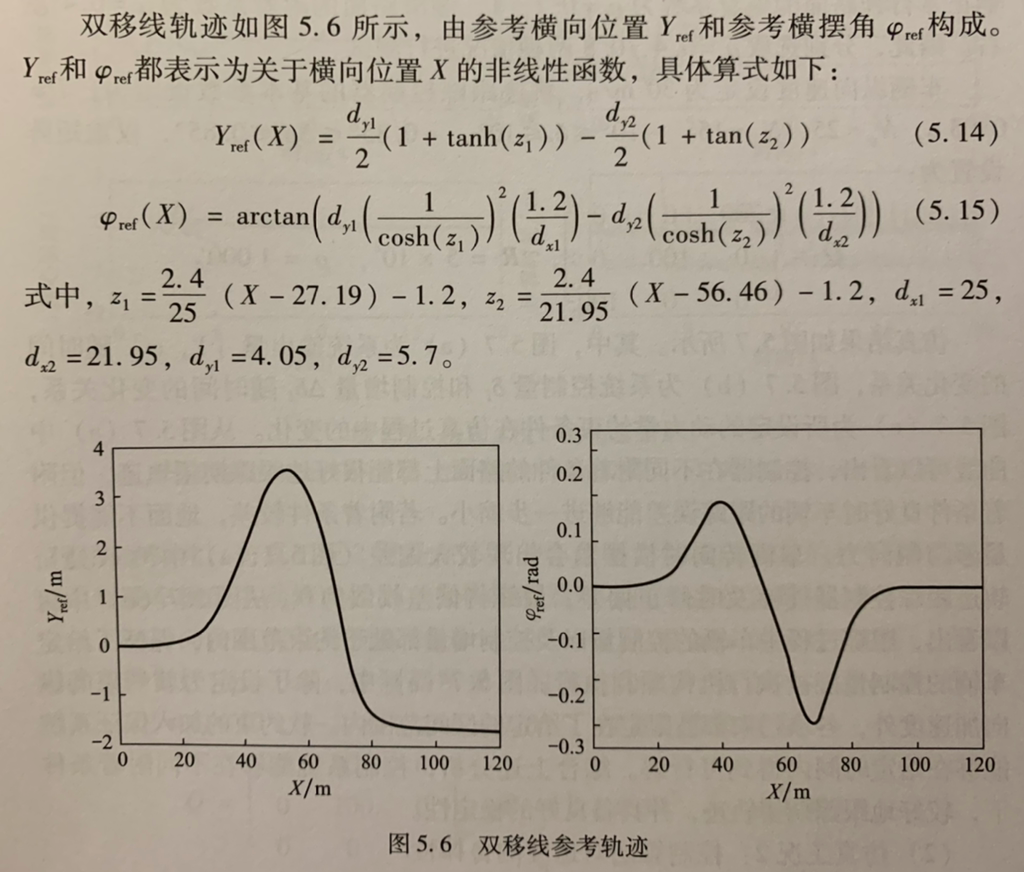
Model predictive controllers based on kinetic models are mainly used for trajectory tracking at higher speeds. In this case the evaluation of the controller is not only the tracking accuracy, but also needs to focus on the stability in the tracking process. In the test of general wheel form stability, the double shift line condition is a common test section. The reference trajectory of the double shift line is shown in the figure below, which consists of the reference transverse position Yref and the reference traverse angle φre, both of which are nonlinear functions of the total longitudinal position Y. The reference trajectory of the double shift line is shown in the figure below:
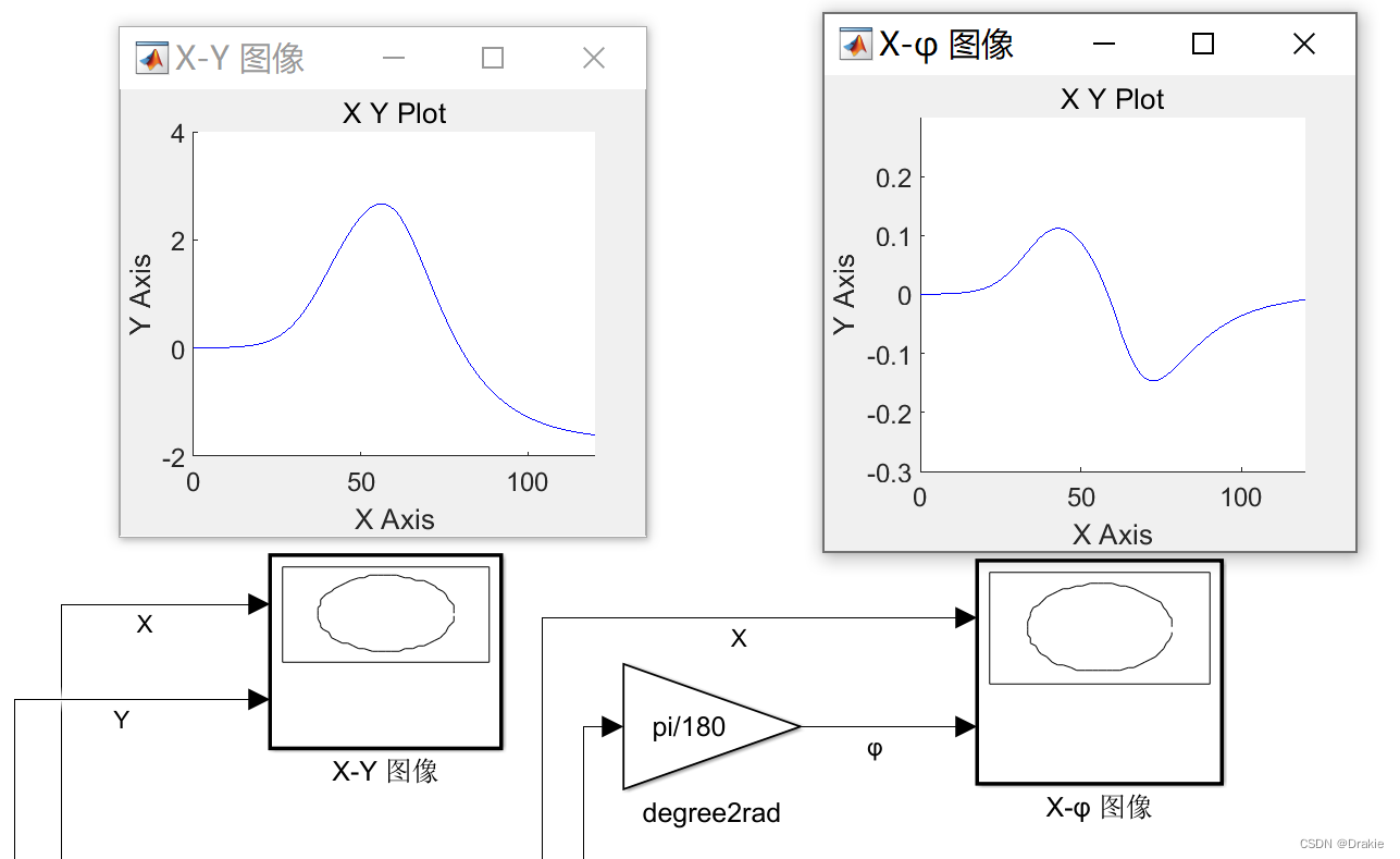
Under the working condition of vehicle speed of 30 km/h and road friction coefficient of 1, the simulation results of trolley trajectory tracking are shown below, and it can be seen that the actual running trajectory is basically the same as that of the double-shifted line trajectory:
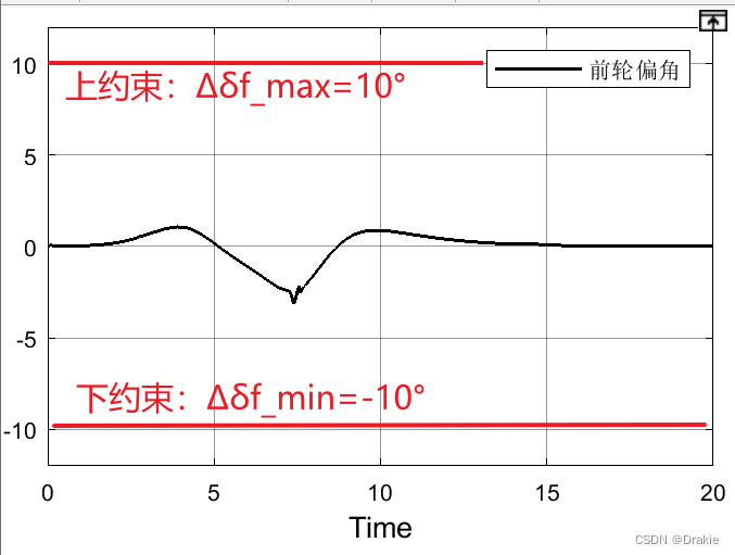
Here you can see that the amount of control is constrained to be within limits
4 Simulation results under different operating conditions
The designed active steering tracking controller takes the front wheel deflection of the vehicle as an input to the controller and the control objective is to track the reference trajectory by continuously reducing the deviation from the reference trajectory.
4.1 Robustness of the control system to pavement adhesion conditions
When a driverless vehicle is driving on roads with different attachment conditions (e.g., dry road, wet road), the vehicle’s own dynamics parameters, such as tire lateral deflection stiffness, will change, and there will also be insufficient lateral force provided by the ground. This brings some challenges to the performance of the controller.
If the attachment conditions are poor, the ground can not provide enough lateral force, the vehicle steering swing angle will appear a large deviation, the trajectory tracking controller can correct the deviation in a timely manner, and finally converge the deviation to 0. And the control amount and control increment of the vehicle in the tracking process are within the constraint range. The addition of soft constraints can ensure that the system can get a feasible solution in a given time, so the control system can track the desired trajectory better under different attachment conditions and has good stability.
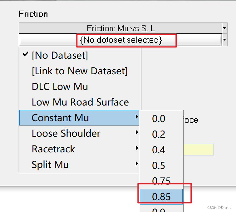
Carsim Pavement Adhesion Factor Modification Guide:

Choose the coefficient of adhesion, usually dry road coefficient of adhesion of 0.7 ~ 1, slippery road coefficient of adhesion of about 0.4
4.2 Robustness of the control algorithm to velocity
While many controllers often need to determine different control parameters for different driving speeds, model predictive controllers are able to predict the future output of the system based on the established vehicle model and are robust to changes in vehicle speed.
The simulation experiments of active steering system were driven at 10m/s 20m/s and 30m/s respectively, with good road adhesion conditions and an adhesion coefficient of 0.8, and the parameters used for the controller were T=0.05, Np=15, and Nc=10.
From the results, it can be seen that the higher the speed, the larger the increment of the control volume, but not exceeding the constraint range. The dynamics constraints remain within the interval range, while the center of mass lateral deflection is well below the limit range, indicating that the vehicle travels very smoothly and the increase in speed does not lead to a decrease in the stability of the vehicle.
4.3 Effect of different design parameters on the controller
The impact of different parameters on the performance of the controller varies. For model predictive controllers, the most important design parameters are the prediction time domain and control time domain. The use of smaller prediction and control time domains leads to larger tracking deviations, but is effective in improving the real-time performance of the control system.

