Machine Learning for Localized Path Planning

This blog series includes six columns, namely: Overview of Autonomous Driving Technology, Fundamentals of Autonomous Vehicle Platform Technology, Autonomous Vehicle Positioning Technology, Autonomous Vehicle Environment Sensing, Autonomous Vehicle Decision Making and Control, and Autonomous Vehicle System Design and Applications.
This column is about notes from the book Decision Making and Control of Self-Driving Vehicles.

---

---

2. Automobile local trajectory planning

2.4 Application of Machine Learning to Localized Path Planning

1. summarize

   • Modeling Learning

     The state-action mapping relationship can be obtained by learning in expert example data; however, this learning lacks overall knowledge of the environment and is only applicable to limited or simple scenarios, and also requires the collection of a large amount of data for training, where the quality, quantity, and coverage of the data are very important for imitation learning;

   • Optimization based on excitation function

     Such methods discretize the space into different rasters before applying search methods such as dynamic programming or other mathematical optimization means, where the incentive/cost function is provided by expert data or obtained through inverse augmentation learning;

   • Reverse enhancement learning

     Inverse Reinforcement Learning (IRL) learns to obtain an excitation function by comparing expert example data with a generated trajectory or a strategy for optimizing the excitation function;

     The incentive function can be learned to be obtained by means of expectation feature matching, or the process can be extended directly to the broader optimization problem of maximizing boundary conditions; optimization by feature expectation matching is very ambiguous and requires optimization strategies located in the policy subspace, where the behavior in the policy space is not optimal but still matches the example behavior;

   • Difficulties in applying learning-based methods to the autopilot motion planning problem:

     • Autonomous driving systems need to ensure the safety of public road traffic, which is important during training and testing, and many learning-based approaches require sufficient online training to gather sufficient feedback data from the actual driving environment, a process that has the potential to jeopardize road safety;
     • The reproduction of autonomous driving data is difficult; expert driving data in different scenarios is easy to collect, but it is difficult to reproduce it in a simulation environment because this part of the data contains complex interactions between the main vehicle and its surroundings;
     • Autonomous driving motion planners not only need to cope with dynamically changing and complex traffic environments, but also need to follow traffic rules at every moment, and augmented learning to systematically integrate these constraints is very difficult;

2. Optimal Trajectory Training Based on Augmented Learning

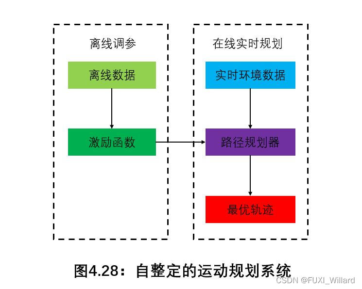
   A self-tuning motion planning system based on Baidu Apollo platform is presented as an example.

   • The online module is responsible for trajectory optimization based on a given excitation function while satisfying the constraints;

   • The motion planning module does not have to be limited to a specific methodology, as trajectories can be generated using sampling-based optimization, dynamic programming, or even augmented learning; however, these planning methods will be evaluated by quantitatively analyzing their optimality and robustness matrices, where optimality is measured by the difference between the optimized trajectory and the value of the excitation function of the generated trajectory, and robustness by the variance of the generated trajectory for a given scenario; on this basis, a final test of the motion planning module’s functionality is provided through simulation and road tests. On this basis, a final test of the functionality of the motion planning module is provided by simulation and road testing;

   • The offline tuning module is responsible for generating incentive/cost functions that can be applied to different driving scenarios; the incentive/cost functions contain characterization factors describing the smoothness of the trajectory and the interaction between the vehicle and the environment, and can be tuned through simulation and road tests;
     

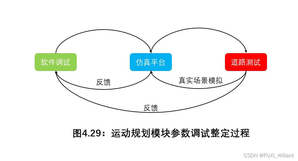
     • The effectiveness of the test parameters needs to be verified by simulation and road tests, and the feedback session is the most time-consuming, requiring verification of parameter performance in thousands of driving scenarios;
     • These driving scenarios include: cities, highways, congested roads, etc., in order to debug to get the incentive function to satisfy these different scenarios, the traditional way of thinking: expanding this process from simple scenarios to complex scenarios, this way, if the current parameter is not good enough for the new scenario, it is necessary to further debug the parameters or even expand the parameter range, and the tuning efficiency is very inefficient; if we use a sequence-based conditional inverse augmented learning framework to target the parameter tuning of the incentive/cost function for autopilot motion planning, it can have very good results;

   • The process of online trajectory evaluation and offline excitation function training is shown below:
     
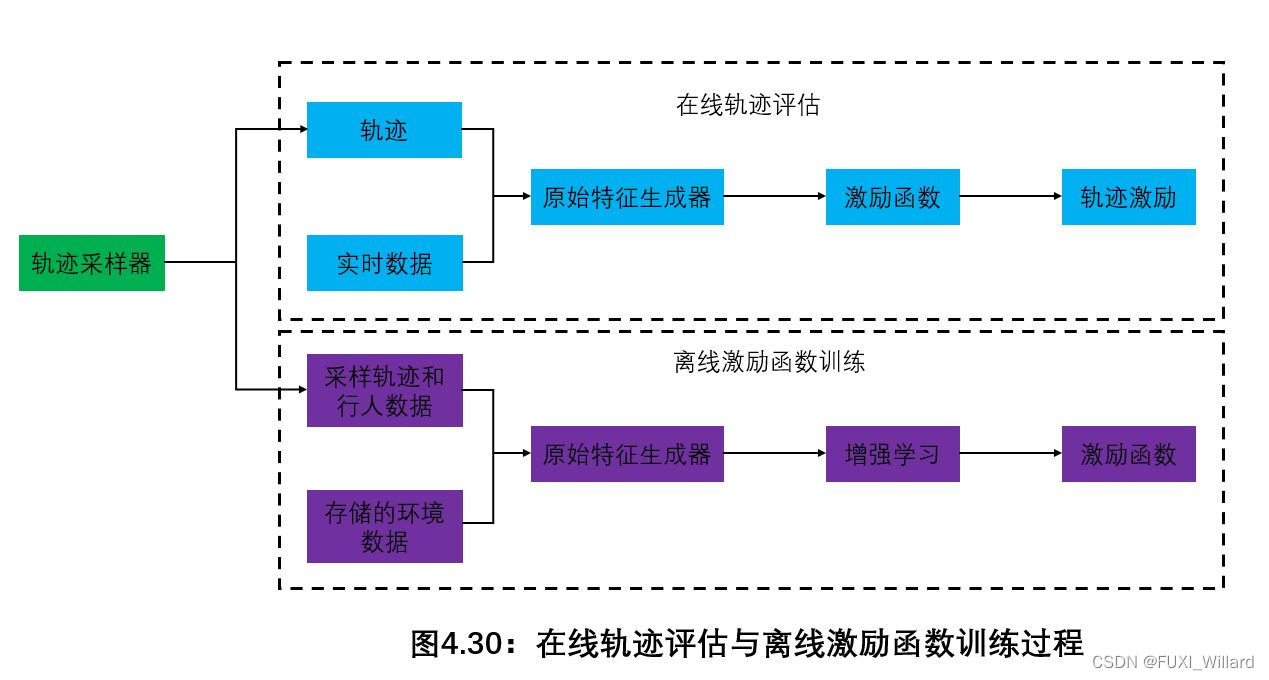
     Raw feature generation takes environmental data as input and evaluates trajectory data sampled or taken from human experts, and the trajectory sampling tool provides candidate trajectories for both online and offline modules;

     In the online evaluation module, after extracting the original features from the trajectories, the incentive/cost function scores and ranks them, and the trajectory with the highest score is output as the final trajectory;

   • The excitation/cost function parameter training is implemented based on the SIAMESE network structure.

     Trajectory characterization based on Markov decision making:$\xi =(a_0,s_0,\dots ,a_N,s_N)\in \Xi$Space$\Xi$is the trajectory sampling space; the initial state of the trajectory is evaluated by the following value function:
     $$V^{\xi }(s_0)=\sum _{t=1}^N{\gamma }_{t}R(a_t,s_t)\text{\hspace{1em}(40)}$$
     This value function is a linear combination of the values of the excitation function at different moment points; the raw feature generation module provides a set of features based on the current state and action, which are summarized in a$f_j(a_t,s_t),j=1,2,\dots ,K$To express it; choose the following excitation function$R$As all features and parameters$\theta \in \Omega$The function of the
     $$R_{\theta }(a_t,s_t)=\tilde{R}(f_1,f_2,\dots ,f_K,\theta )\text{\hspace{1em}(41)}$$
     $\tilde{R}$It can be a linear combination of all features, or alternatively, a neural network relationship with features as inputs, and this neural network can be considered as a coding process to further acquire the internal features of the state-action mapping; this training process is called RC-IRL;
     
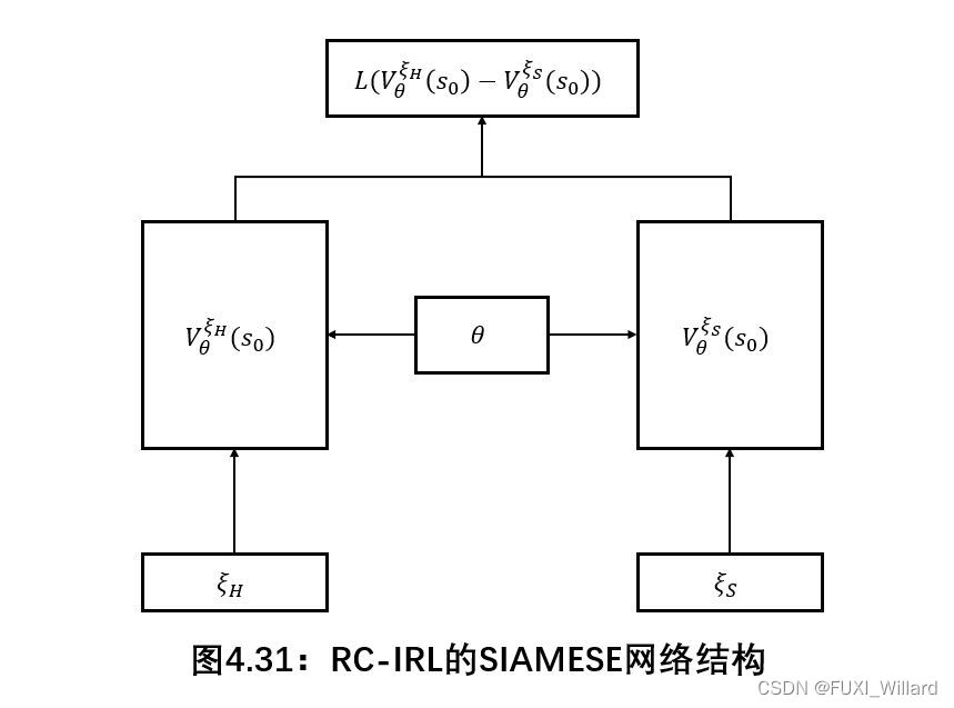
     Among them:${\xi }_H$Demonstrating data on behalf of human experts.${\xi }_S$Delegate space$\Xi$The randomly generated sampling trajectories under the

   • The loss function is a non-negative real function used to quantify the difference between the model predictions and the true labels, and the process of minimizing the loss function is the process of iterating over the parameters so that the cost of a human driving trajectory is less than the cost of a randomly sampled trajectory;

     The loss function is defined as follows, the$a=0.05$：
     $$L(y)=\{\begin{array}{ll}y,& y\ge 0\\ ay,& y<0\end{array}\text{\hspace{1em}(42)}$$
     The structure of the value function training network is shown below: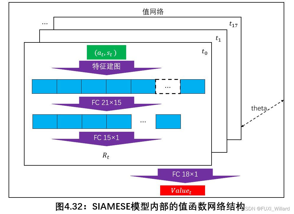