Wise Target Detection 66 – Pytorch builds YoloV8 target detection platform

Preface to the study

Got another YoloV8, looks like it’s grabbing the name.

Source Code Download

https://github.com/bubbliiiing/yolov8–pytorch
If you like it, you can click STAR.

YoloV8 Improvements (incomplete)

A lot of the details don’t have much to do with the YoloV7, probably because it wasn’t developed by the same team.

1, the backbone part: with the previous YoloV5 series gap is not big, but compared to the previous first convolution of the convolution kernel shrinks, is 3 instead of 6. In addition, the preprocessing of the CSP module from three times the convolution of two convolutions, the specific implementation of the first convolution of the number of channels expanded to twice the original, and then convolution of the results of the channel on the half split. In addition, the multi-stacking structure of YoloV7 is borrowed.

2, strengthen the feature extraction part: no longer on the backbone network to obtain the feature layer convolution (the purpose is estimated to speed up), in addition to the CSP module of the preprocessing from the three times the convolution of the two convolution, the realization of the same way as the backbone network.

3, the prediction header: added the DFL module, the DFL module is simply understood as a probabilistic way to obtain the regression value, for example, we currently set the length of the DFL is 8, then a certain regression value is calculated as:

The prediction results are taken as softmax	0.0	0.1	0.0	0.0	0.4	0.5	0.0	0.0	multiply (mathematics)
Fixed value for reference	0	1	2	3	4	5	6	7	0.1 * 1 + 0.4 * 4 + 0.5 * 5 = 4.2

That is, the predicted probability is dot-multiplied with range(0,8) to obtain the regression value. In YoloV8, the length of the DFL is 16, and there are a total of four targets to be regressed, so the channel of the regression header is 16$\times$ 4 = 64。

4, adaptive multiple positive sample matching: in YoloV8, reference to YoloX using the implementation of no anchors, is an anchorless algorithm, the face of irregular length and width of the target is more advantageous; in the calculation of the loss of positive sample matching, the positive samples need to meet the two conditions: one is in the real box, the second is the real box topk the most compliant positive samples (predicted box and the real box overlap) degree is high and the species prediction is accurate).

The above is not the whole part of the improvements, there are some other improvements, here is only a list of some of the ones that I am more interested in and that are very effective.

YoloV8 Implementation Ideas

I. Overall structural analysis

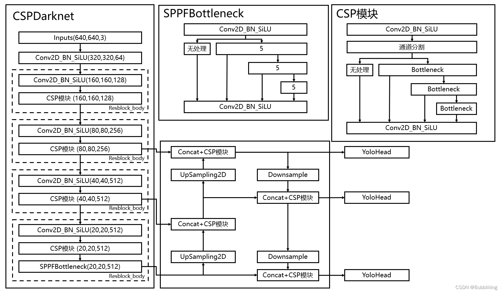
Before learning about YoloV8, we need to have some understanding of what YoloV8 does, which will help us go into the details of the network later. YoloV8 is not much different from the previous Yolo in the way it predicts, and is still divided into three parts.

Backbone, FPN and Yolo Head, respectively.。

Backbone is the backbone feature extraction network of YoloV8The input image is first processed inside the backbone network.feature extraction, the extracted features can be referred to as feature layers.is the set of features of the input image. In the main section, weThree feature layers were acquiredTo carry out the next step in the construction of the network, these three feature layers I call itEffective feature layer。

FPN is an enhanced feature extraction network for YoloV8The three that were obtained in the main part of theEffective feature layerWill perform feature fusion in this section, the purpose of feature fusion is to combine feature information from different scales. In the FPN section, the acquiredEffective feature layerwas used to continue extracting features.In YoloV8, the Panet structure is still used, where we not only up-sample the features to achieve feature fusion, but also down-sample them again to achieve feature fusion.

Yolo Head is a classifier and regressor for YoloV8The FPN and the Backbone have allowed us to obtain three enhanced and effective feature layers. Each feature layer has width, height, and number of channels, at which point we can set theThe feature map is viewed as a collection of feature points one after anotherthat each feature point serves as a prior point and that there is no longer a prior frame.Each a priori point has channel number of featuresWhat Yolo Head is actually doing isJudgment of feature pointsjudgementWhether the a priori frame on the feature point has an object corresponding to itThe decoupling header used by YoloV8 is separate, i.e., classification and regression are not implemented in a single 1X1 convolution.

Thus, the work done by the entire YoloV8 network remains the sameFeature Extraction-Feature Enhancement-Prediction of Object Situations Corresponding to A Priori Frames。

II. Network structure analysis

1. Introduction to Backbone, the backbone network

The backbone feature extraction network used by YoloV8 has been optimized mainly for speed:
1, the neck structure uses a normal 3×3 convolution with a step size of 2.
Previously:
YoloV5 initially used the Focus structure for initial feature extraction, and in an improved version used convolution with a large convolutional kernel for initial feature extraction, neither of which was fast.
YoloV7, on the other hand, uses three convolutions to initially extract features, and is not as fast.
YoloV8, on the other hand, uses a normal 3×3 convolutional kernel with a step size of 2 to initially extract the features (presumably with enough feeler fields).

self.stem = Conv(3, base_channels, 3, 2)

This loses some feeler field, but improves the speed of the model.

2, the preprocessing of the CSP module was switched from three convolutions to two, and the multi-stacking structure of YoloV7 was borrowed.
The specific implementation is to expand the number of channels for the first convolution to twice the original number, and then split the convolution result in half on the channel, which can reduce the number of times of one convolution and speed up the network.

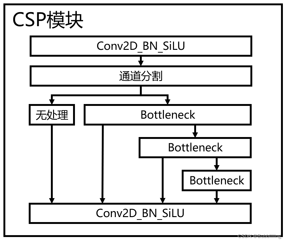
The realization code is as follows:

class C2f(nn.Module):
    # CSPNet structure structure, large residual structure
    # c1 is the number of input channels, c2 is the number of output channels
    def __init__(self, c1, c2, n=1, shortcut=False, g=1, e=0.5):
        super().__init__()
        self.c      = int(c2 * e) 
        self.cv1    = Conv(c1, 2 * self.c, 1, 1)
        self.cv2    = Conv((2 + n) * self.c, c2, 1)
        self.m      = nn.ModuleList(Bottleneck(self.c, self.c, shortcut, g, k=((3, 3), (3, 3)), e=1.0) for _ in range(n))

    def forward(self, x):
        # Perform a convolution and then divide into two, each channel being c
        y = list(self.cv1(x).split((self.c, self.c), 1))
        # Residual structures are retained for each carry and then stacked together, dense residuals
        y.extend(m(y[-1]) for m in self.m)
        return self.cv2(torch.cat(y, 1))

The entire backbone implementation code is:

import torch
import torch.nn as nn


def autopad(k, p=None, d=1):  
    # kernel, padding, dilation
    # Perform automatic padding on the input feature layer, following the Same principle
    if d > 1:
        # actual kernel-size
        k = d * (k - 1) + 1 if isinstance(k, int) else [d * (x - 1) + 1 for x in k]
    if p is None:
        # auto-pad
        p = k // 2 if isinstance(k, int) else [x // 2 for x in k]
    return p

class SiLU(nn.Module):  
    # SiLU activation function
    @staticmethod
    def forward(x):
        return x * torch.sigmoid(x)
    
class Conv(nn.Module):
    # Standard convolution + normalization + activation function
    default_act = SiLU() 
    def __init__(self, c1, c2, k=1, s=1, p=None, g=1, d=1, act=True):
        super().__init__()
        self.conv   = nn.Conv2d(c1, c2, k, s, autopad(k, p, d), groups=g, dilation=d, bias=False)
        self.bn     = nn.BatchNorm2d(c2, eps=0.001, momentum=0.03, affine=True, track_running_stats=True)
        self.act    = self.default_act if act is True else act if isinstance(act, nn.Module) else nn.Identity()

    def forward(self, x):
        return self.act(self.bn(self.conv(x)))

    def forward_fuse(self, x):
        return self.act(self.conv(x))

class Bottleneck(nn.Module):
    # Standard bottleneck structure, residual structure
    # c1 is the number of input channels, c2 is the number of output channels
    def __init__(self, c1, c2, shortcut=True, g=1, k=(3, 3), e=0.5):
        super().__init__()
        c_ = int(c2 * e)  # hidden channels
        self.cv1 = Conv(c1, c_, k[0], 1)
        self.cv2 = Conv(c_, c2, k[1], 1, g=g)
        self.add = shortcut and c1 == c2

    def forward(self, x):
        return x + self.cv2(self.cv1(x)) if self.add else self.cv2(self.cv1(x))    

class C2f(nn.Module):
    # CSPNet structure structure, large residual structure
    # c1 is the number of input channels, c2 is the number of output channels
    def __init__(self, c1, c2, n=1, shortcut=False, g=1, e=0.5):
        super().__init__()
        self.c      = int(c2 * e) 
        self.cv1    = Conv(c1, 2 * self.c, 1, 1)
        self.cv2    = Conv((2 + n) * self.c, c2, 1)
        self.m      = nn.ModuleList(Bottleneck(self.c, self.c, shortcut, g, k=((3, 3), (3, 3)), e=1.0) for _ in range(n))

    def forward(self, x):
        # Perform a convolution and then divide into two, each channel being c
        y = list(self.cv1(x).split((self.c, self.c), 1))
        # Residual structures are retained for each carry and then stacked together, dense residuals
        y.extend(m(y[-1]) for m in self.m)
        return self.cv2(torch.cat(y, 1))
    
class SPPF(nn.Module):
    # SPP structure, 5, 9, 13 Maximum pooling of maximal pooling kernels.
    def __init__(self, c1, c2, k=5):
        super().__init__()
        c_          = c1 // 2
        self.cv1    = Conv(c1, c_, 1, 1)
        self.cv2    = Conv(c_ * 4, c2, 1, 1)
        self.m      = nn.MaxPool2d(kernel_size=k, stride=1, padding=k // 2)

    def forward(self, x):
        x = self.cv1(x)
        y1 = self.m(x)
        y2 = self.m(y1)
        return self.cv2(torch.cat((x, y1, y2, self.m(y2)), 1))

class Backbone(nn.Module):
    def __init__(self, base_channels, base_depth, deep_mul, phi, pretrained=False):
        super().__init__()
        #-----------------------------------------------#
        # Input image is 3, 640, 640
        #-----------------------------------------------#
        # 3, 640, 640 => 32, 640, 640 => 64, 320, 320
        self.stem = Conv(3, base_channels, 3, 2)
        
        # 64, 320, 320 => 128, 160, 160 => 128, 160, 160
        self.dark2 = nn.Sequential(
            Conv(base_channels, base_channels * 2, 3, 2),
            C2f(base_channels * 2, base_channels * 2, base_depth, True),
        )
        # 128, 160, 160 => 256, 80, 80 => 256, 80, 80
        self.dark3 = nn.Sequential(
            Conv(base_channels * 2, base_channels * 4, 3, 2),
            C2f(base_channels * 4, base_channels * 4, base_depth * 2, True),
        )
        # 256, 80, 80 => 512, 40, 40 => 512, 40, 40
        self.dark4 = nn.Sequential(
            Conv(base_channels * 4, base_channels * 8, 3, 2),
            C2f(base_channels * 8, base_channels * 8, base_depth * 2, True),
        )
        # 512, 40, 40 => 1024 * deep_mul, 20, 20 => 1024 * deep_mul, 20, 20
        self.dark5 = nn.Sequential(
            Conv(base_channels * 8, int(base_channels * 16 * deep_mul), 3, 2),
            C2f(int(base_channels * 16 * deep_mul), int(base_channels * 16 * deep_mul), base_depth, True),
            SPPF(int(base_channels * 16 * deep_mul), int(base_channels * 16 * deep_mul), k=5)
        )
        
        if pretrained:
            url = {
                "n" : 'https://github.com/bubbliiiing/yolov8-pytorch/releases/download/v1.0/yolov8_n_backbone_weights.pth',
                "s" : 'https://github.com/bubbliiiing/yolov8-pytorch/releases/download/v1.0/yolov8_s_backbone_weights.pth',
                "m" : 'https://github.com/bubbliiiing/yolov8-pytorch/releases/download/v1.0/yolov8_m_backbone_weights.pth',
                "l" : 'https://github.com/bubbliiiing/yolov8-pytorch/releases/download/v1.0/yolov8_l_backbone_weights.pth',
                "x" : 'https://github.com/bubbliiiing/yolov8-pytorch/releases/download/v1.0/yolov8_x_backbone_weights.pth',
            }[phi]
            checkpoint = torch.hub.load_state_dict_from_url(url=url, map_location="cpu", model_dir="./model_data")
            self.load_state_dict(checkpoint, strict=False)
            print("Load weights from " + url.split('/')[-1])

    def forward(self, x):
        x = self.stem(x)
        x = self.dark2(x)
        #-----------------------------------------------#
        # dark3's output is 256, 80, 80, a valid feature layer
        #-----------------------------------------------#
        x = self.dark3(x)
        feat1 = x
        #-----------------------------------------------#
        # dark4's output of 512, 40, 40 is a valid feature layer
        #-----------------------------------------------#
        x = self.dark4(x)
        feat2 = x
        #-----------------------------------------------#
        # dark5's output is 1024 * deep_mul, 20, 20, a valid feature layer
        #-----------------------------------------------#
        x = self.dark5(x)
        feat3 = x
        return feat1, feat2, feat3

2. construct FPN feature pyramid for enhanced feature extraction

In the feature utilization section, YoloV8 extracts theMultiple feature layers for target detectionTotalExtraction of three feature layers。
The three feature layers are located at different locations in the main trunk section of theMiddle, Lower Middle, Bottom, when the input is (640,640,3), the three feature layers of theThe shapes are feature1 = (80,80,256), feature2 = (40,40,512), and feature3 = (20,20,1024 * deep_mul) respectively。

deep_mul is just a coefficient that scales the deeper channels, which in YoloV8 is supposed to be a consideration made to balance the amount of computation.

After obtaining the three effective feature layers, we utilize these three effective feature layers for the construction of the FPN layer, which is constructed as follows (in this blog post, the SPPCSPC structure is subsumed in the FPN):

1. The feature layer feature3=(20,20,512) is up-sampled UmSampling2d and then combined with the feature layer feature2=(40,40,512), and then feature extraction is performed using the CSP module to obtain P4, at which point the feature layer obtained is (40,40,512).
2. P4=(40,40,512) is upsampled UmSampling2d and then combined with feature1=(80,80,256) feature layer, and then the CSP module is used for feature extraction to obtain P3, at which point the feature layer obtained is (80,80,256).
3. The feature layer of P3=(80,80,256) is downsampled by one 3×3 convolution ofDownsampled and stacked with P4, and then the CSP module is used for feature extraction to obtain the new P4, at which point the obtained feature layer is (40,40,512).
4. The feature layer of P4=(40,40,512) is downsampled by one 3×3 convolution ofDownsampled and stacked with P5, and then the CSP module is used for feature extraction to obtain the new P5, at which point the feature layer obtained is (20,20,1024 * deep_mul).

The feature pyramid allows for the integration ofFeature fusion of feature layers from different shapesIn favor ofExtracting better features。

#---------------------------------------------------#
#   yolo_body
#---------------------------------------------------#
class YoloBody(nn.Module):
    def __init__(self, input_shape, num_classes, phi, pretrained=False):
        super(YoloBody, self).__init__()
        depth_dict          = {'n' : 0.33, 's' : 0.33, 'm' : 0.67, 'l' : 1.00, 'x' : 1.00,}
        width_dict          = {'n' : 0.25, 's' : 0.50, 'm' : 0.75, 'l' : 1.00, 'x' : 1.25,}
        deep_width_dict     = {'n' : 1.00, 's' : 1.00, 'm' : 0.75, 'l' : 0.50, 'x' : 0.50,}
        dep_mul, wid_mul, deep_mul = depth_dict[phi], width_dict[phi], deep_width_dict[phi]

        base_channels       = int(wid_mul * 64)  # 64
        base_depth          = max(round(dep_mul * 3), 1)  # 3
        #-----------------------------------------------#
        # Input image is 3, 640, 640
        #-----------------------------------------------#

        #---------------------------------------------------#   
        # Generate backbone models
        # Three valid feature layers are obtained and their shapes are:
        #   256, 80, 80
        #   512, 40, 40
        #   1024 * deep_mul, 20, 20
        #---------------------------------------------------#
        self.backbone   = Backbone(base_channels, base_depth, deep_mul, phi, pretrained=pretrained)

        #------------------------ Enhanced Feature Extraction Network ------------------------# 
        self.upsample   = nn.Upsample(scale_factor=2, mode="nearest")

        # 1024 * deep_mul + 512, 40, 40 => 512, 40, 40
        self.conv3_for_upsample1    = C2f(int(base_channels * 16 * deep_mul) + base_channels * 8, base_channels * 8, base_depth, shortcut=False)
        # 768, 80, 80 => 256, 80, 80
        self.conv3_for_upsample2    = C2f(base_channels * 8 + base_channels * 4, base_channels * 4, base_depth, shortcut=False)
        
        # 256, 80, 80 => 256, 40, 40
        self.down_sample1           = Conv(base_channels * 4, base_channels * 4, 3, 2)
        # 512 + 256, 40, 40 => 512, 40, 40
        self.conv3_for_downsample1  = C2f(base_channels * 8 + base_channels * 4, base_channels * 8, base_depth, shortcut=False)

        # 512, 40, 40 => 512, 20, 20
        self.down_sample2           = Conv(base_channels * 8, base_channels * 8, 3, 2)
        # 1024 * deep_mul + 512, 20, 20 =>  1024 * deep_mul, 20, 20
        self.conv3_for_downsample2  = C2f(int(base_channels * 16 * deep_mul) + base_channels * 8, int(base_channels * 16 * deep_mul), base_depth, shortcut=False)
        #------------------------ Enhanced Feature Extraction Network ------------------------# 
        
        ch              = [base_channels * 4, base_channels * 8, int(base_channels * 16 * deep_mul)]
        self.shape      = None
        self.nl         = len(ch)
        # self.stride     = torch.zeros(self.nl)
        self.stride     = torch.tensor([256 / x.shape[-2] for x in self.backbone.forward(torch.zeros(1, 3, 256, 256))])  # forward
        self.reg_max    = 16  # DFL channels (ch[0] // 16 to scale 4/8/12/16/20 for n/s/m/l/x)
        self.no         = num_classes + self.reg_max * 4  # number of outputs per anchor
        self.num_classes = num_classes
        
        c2, c3   = max((16, ch[0] // 4, self.reg_max * 4)), max(ch[0], num_classes)  # channels
        self.cv2 = nn.ModuleList(nn.Sequential(Conv(x, c2, 3), Conv(c2, c2, 3), nn.Conv2d(c2, 4 * self.reg_max, 1)) for x in ch)
        self.cv3 = nn.ModuleList(nn.Sequential(Conv(x, c3, 3), Conv(c3, c3, 3), nn.Conv2d(c3, num_classes, 1)) for x in ch)
        self.dfl = DFL(self.reg_max) if self.reg_max > 1 else nn.Identity()


    def fuse(self):
        print('Fusing layers... ')
        for m in self.modules():
            if type(m) is Conv and hasattr(m, 'bn'):
                m.conv = fuse_conv_and_bn(m.conv, m.bn)  # update conv
                delattr(m, 'bn')  # remove batchnorm
                m.forward = m.forward_fuse  # update forward
        return self
    
    def forward(self, x):
        #  backbone
        feat1, feat2, feat3 = self.backbone.forward(x)
        
        #------------------------ Enhanced Feature Extraction Network ------------------------# 
        # 1024 * deep_mul, 20, 20 => 1024 * deep_mul, 40, 40
        P5_upsample = self.upsample(feat3)
        # 1024 * deep_mul, 40, 40 cat 512, 40, 40 => 1024 * deep_mul + 512, 40, 40
        P4          = torch.cat([P5_upsample, feat2], 1)
        # 1024 * deep_mul + 512, 40, 40 => 512, 40, 40
        P4          = self.conv3_for_upsample1(P4)

        # 512, 40, 40 => 512, 80, 80
        P4_upsample = self.upsample(P4)
        # 512, 80, 80 cat 256, 80, 80 => 768, 80, 80
        P3          = torch.cat([P4_upsample, feat1], 1)
        # 768, 80, 80 => 256, 80, 80
        P3          = self.conv3_for_upsample2(P3)

        # 256, 80, 80 => 256, 40, 40
        P3_downsample = self.down_sample1(P3)
        # 512, 40, 40 cat 256, 40, 40 => 768, 40, 40
        P4 = torch.cat([P3_downsample, P4], 1)
        # 768, 40, 40 => 512, 40, 40
        P4 = self.conv3_for_downsample1(P4)

        # 512, 40, 40 => 512, 20, 20
        P4_downsample = self.down_sample2(P4)
        # 512, 20, 20 cat 1024 * deep_mul, 20, 20 => 1024 * deep_mul + 512, 20, 20
        P5 = torch.cat([P4_downsample, feat3], 1)
        # 1024 * deep_mul + 512, 20, 20 => 1024 * deep_mul, 20, 20
        P5 = self.conv3_for_downsample2(P5)
        #------------------------ Enhanced Feature Extraction Network ------------------------# 
        # P3 256, 80, 80
        # P4 512, 40, 40
        # P5 1024 * deep_mul, 20, 20
        shape = P3.shape  # BCHW
        
        # P3 256, 80, 80 => num_classes + self.reg_max * 4, 80, 80
        # P4 512, 40, 40 => num_classes + self.reg_max * 4, 40, 40
        # P5 1024 * deep_mul, 20, 20 => num_classes + self.reg_max * 4, 20, 20
        x = [P3, P4, P5]
        for i in range(self.nl):
            x[i] = torch.cat((self.cv2[i](x[i]), self.cv3[i](x[i])), 1)

        if self.shape != shape:
            self.anchors, self.strides = (x.transpose(0, 1) for x in make_anchors(x, self.stride, 0.5))
            self.shape = shape
        
        # num_classes + self.reg_max * 4 , 8400 =>  cls num_classes, 8400; 
        #                                           box self.reg_max * 4, 8400
        box, cls        = torch.cat([xi.view(shape[0], self.no, -1) for xi in x], 2).split((self.reg_max * 4, self.num_classes), 1)
        # origin_cls      = [xi.split((self.reg_max * 4, self.num_classes), 1)[1] for xi in x]
        dbox            = self.dfl(box)
        return dbox, cls, x, self.anchors.to(dbox.device), self.strides.to(dbox.device)

3. Use Yolo Head to obtain predicted results

Using the FPN feature pyramid, theWe can obtain three reinforcing features, which have the shapes of (20,20,1024 * deep_mul), (40,40,512), (80,80,256), and then we utilize the feature layers of these three shapes to pass into the Yolo Head to obtain the prediction results, YoloV8 uses a decoupled head and uses the DFL technique.

Unlike the previous Yolo series, YoloV8 uses a DFL structure after Yolo Head to compute the regression values instead of obtaining them directly.The DFL module is simply understood to obtain regression values in a probabilistic manner, for example, if we currently set the length of the DFL to 8, then a certain regression value is calculated as:

The prediction results are taken as softmax	0.0	0.1	0.0	0.0	0.4	0.5	0.0	0.0	multiply (mathematics)
Fixed value for reference	0	1	2	3	4	5	6	7	0.1 * 1 + 0.4 * 4 + 0.5 * 5 = 4.2

And for each feature layer, we can obtain the kinds and regression values of the corresponding prediction frames for each feature point target using two independent convolutional adjustments of the number of channels, respectively.The number of channels of the regression value-dependent predictor header is related to the length of the DFL, which is set to 16 in YoloV8, and the number of channels of the species-dependent predictor header is related to the number of species to be differentiated。

Regardless of the dataset used, the number of channels of the prediction header associated with the regression values is$16\times 4=64$, the shapes of the three feature layers are (20,20,64)，(40,40,64)，(80,80,64). 64 can be divided into four 16 for the calculation of the four regression coefficients.
After calculating the regression coefficients. The shapes of the three feature layers are (20,20,4)，(40,40,4)，(80,80,4)

If the voc training set is used, the classes are 20, and the number of channels for the species-related prediction header is 20, the shapes of the three feature layers are (20,20,20)，(40,40,20)，(80,80,20). Used to determine the type of object contained in each feature point.

If the coco training set is used, the classes are 80, and the number of channels for the species-related prediction header is 80, the shapes of the three feature layers are (20,20,80)，(40,40,80)，(80,80,80). Used to determine the type of object contained in each feature point.

The realization code is as follows:

import numpy as np
import torch
import torch.nn as nn
from nets.backbone import Backbone, C2f, Conv, SiLU, autopad
from utils.utils_bbox import make_anchors
def fuse_conv_and_bn(conv, bn):
# Blend Conv2d + BatchNorm2d Reduced computation
# Fuse Conv2d() and BatchNorm2d() layers https://tehnokv.com/posts/fusing-batchnorm-and-conv/
fusedconv = nn.Conv2d(conv.in_channels,
conv.out_channels,
kernel_size=conv.kernel_size,
stride=conv.stride,
padding=conv.padding,
dilation=conv.dilation,
groups=conv.groups,
bias=True).requires_grad_(False).to(conv.weight.device)
# Prepare the kernel
w_conv = conv.weight.clone().view(conv.out_channels, -1)
w_bn = torch.diag(bn.weight.div(torch.sqrt(bn.eps + bn.running_var)))
fusedconv.weight.copy_(torch.mm(w_bn, w_conv).view(fusedconv.weight.shape))
# Prepare bias
b_conv = torch.zeros(conv.weight.size(0), device=conv.weight.device) if conv.bias is None else conv.bias
b_bn = bn.bias - bn.weight.mul(bn.running_mean).div(torch.sqrt(bn.running_var + bn.eps))
fusedconv.bias.copy_(torch.mm(w_bn, b_conv.reshape(-1, 1)).reshape(-1) + b_bn)
return fusedconv
class DFL(nn.Module):
# DFL modules
# Distribution Focal Loss (DFL) proposed in Generalized Focal Loss https://ieeexplore.ieee.org/document/9792391
def __init__(self, c1=16):
super().__init__()
self.conv   = nn.Conv2d(c1, 1, 1, bias=False).requires_grad_(False)
x           = torch.arange(c1, dtype=torch.float)
self.conv.weight.data[:] = nn.Parameter(x.view(1, c1, 1, 1))
self.c1     = c1
def forward(self, x):
# bs, self.reg_max * 4, 8400
b, c, a = x.shape
# bs, 4, self.reg_max, 8400 => bs, self.reg_max, 4, 8400 => b, 4, 8400
# Calculate the percentage for numbers from 0 to 16 in softmax fashion to get the final number.
return self.conv(x.view(b, 4, self.c1, a).transpose(2, 1).softmax(1)).view(b, 4, a)
# return self.conv(x.view(b, self.c1, 4, a).softmax(1)).view(b, 4, a)
#---------------------------------------------------#
#   yolo_body
#---------------------------------------------------#
class YoloBody(nn.Module):
def __init__(self, input_shape, num_classes, phi, pretrained=False):
super(YoloBody, self).__init__()
depth_dict          = {'n' : 0.33, 's' : 0.33, 'm' : 0.67, 'l' : 1.00, 'x' : 1.00,}
width_dict          = {'n' : 0.25, 's' : 0.50, 'm' : 0.75, 'l' : 1.00, 'x' : 1.25,}
deep_width_dict     = {'n' : 1.00, 's' : 1.00, 'm' : 0.75, 'l' : 0.50, 'x' : 0.50,}
dep_mul, wid_mul, deep_mul = depth_dict[phi], width_dict[phi], deep_width_dict[phi]
base_channels       = int(wid_mul * 64)  # 64
base_depth          = max(round(dep_mul * 3), 1)  # 3
#-----------------------------------------------#
# Input image is 3, 640, 640
#-----------------------------------------------#
#---------------------------------------------------#   
# Generate backbone models
# Three valid feature layers are obtained and their shapes are:
#   256, 80, 80
#   512, 40, 40
#   1024 * deep_mul, 20, 20
#---------------------------------------------------#
self.backbone   = Backbone(base_channels, base_depth, deep_mul, phi, pretrained=pretrained)
#------------------------ Enhanced Feature Extraction Network ------------------------# 
self.upsample   = nn.Upsample(scale_factor=2, mode="nearest")
# 1024 * deep_mul + 512, 40, 40 => 512, 40, 40
self.conv3_for_upsample1    = C2f(int(base_channels * 16 * deep_mul) + base_channels * 8, base_channels * 8, base_depth, shortcut=False)
# 768, 80, 80 => 256, 80, 80
self.conv3_for_upsample2    = C2f(base_channels * 8 + base_channels * 4, base_channels * 4, base_depth, shortcut=False)
# 256, 80, 80 => 256, 40, 40
self.down_sample1           = Conv(base_channels * 4, base_channels * 4, 3, 2)
# 512 + 256, 40, 40 => 512, 40, 40
self.conv3_for_downsample1  = C2f(base_channels * 8 + base_channels * 4, base_channels * 8, base_depth, shortcut=False)
# 512, 40, 40 => 512, 20, 20
self.down_sample2           = Conv(base_channels * 8, base_channels * 8, 3, 2)
# 1024 * deep_mul + 512, 20, 20 =>  1024 * deep_mul, 20, 20
self.conv3_for_downsample2  = C2f(int(base_channels * 16 * deep_mul) + base_channels * 8, int(base_channels * 16 * deep_mul), base_depth, shortcut=False)
#------------------------ Enhanced Feature Extraction Network ------------------------# 
ch              = [base_channels * 4, base_channels * 8, int(base_channels * 16 * deep_mul)]
self.shape      = None
self.nl         = len(ch)
# self.stride     = torch.zeros(self.nl)
self.stride     = torch.tensor([256 / x.shape[-2] for x in self.backbone.forward(torch.zeros(1, 3, 256, 256))])  # forward
self.reg_max    = 16  # DFL channels (ch[0] // 16 to scale 4/8/12/16/20 for n/s/m/l/x)
self.no         = num_classes + self.reg_max * 4  # number of outputs per anchor
self.num_classes = num_classes
c2, c3   = max((16, ch[0] // 4, self.reg_max * 4)), max(ch[0], num_classes)  # channels
self.cv2 = nn.ModuleList(nn.Sequential(Conv(x, c2, 3), Conv(c2, c2, 3), nn.Conv2d(c2, 4 * self.reg_max, 1)) for x in ch)
self.cv3 = nn.ModuleList(nn.Sequential(Conv(x, c3, 3), Conv(c3, c3, 3), nn.Conv2d(c3, num_classes, 1)) for x in ch)
self.dfl = DFL(self.reg_max) if self.reg_max > 1 else nn.Identity()
def fuse(self):
print('Fusing layers... ')
for m in self.modules():
if type(m) is Conv and hasattr(m, 'bn'):
m.conv = fuse_conv_and_bn(m.conv, m.bn)  # update conv
delattr(m, 'bn')  # remove batchnorm
m.forward = m.forward_fuse  # update forward
return self
def forward(self, x):
#  backbone
feat1, feat2, feat3 = self.backbone.forward(x)
#------------------------ Enhanced Feature Extraction Network ------------------------# 
# 1024 * deep_mul, 20, 20 => 1024 * deep_mul, 40, 40
P5_upsample = self.upsample(feat3)
# 1024 * deep_mul, 40, 40 cat 512, 40, 40 => 1024 * deep_mul + 512, 40, 40
P4          = torch.cat([P5_upsample, feat2], 1)
# 1024 * deep_mul + 512, 40, 40 => 512, 40, 40
P4          = self.conv3_for_upsample1(P4)
# 512, 40, 40 => 512, 80, 80
P4_upsample = self.upsample(P4)
# 512, 80, 80 cat 256, 80, 80 => 768, 80, 80
P3          = torch.cat([P4_upsample, feat1], 1)
# 768, 80, 80 => 256, 80, 80
P3          = self.conv3_for_upsample2(P3)
# 256, 80, 80 => 256, 40, 40
P3_downsample = self.down_sample1(P3)
# 512, 40, 40 cat 256, 40, 40 => 768, 40, 40
P4 = torch.cat([P3_downsample, P4], 1)
# 768, 40, 40 => 512, 40, 40
P4 = self.conv3_for_downsample1(P4)
# 512, 40, 40 => 512, 20, 20
P4_downsample = self.down_sample2(P4)
# 512, 20, 20 cat 1024 * deep_mul, 20, 20 => 1024 * deep_mul + 512, 20, 20
P5 = torch.cat([P4_downsample, feat3], 1)
# 1024 * deep_mul + 512, 20, 20 => 1024 * deep_mul, 20, 20
P5 = self.conv3_for_downsample2(P5)
#------------------------ Enhanced Feature Extraction Network ------------------------# 
# P3 256, 80, 80
# P4 512, 40, 40
# P5 1024 * deep_mul, 20, 20
shape = P3.shape  # BCHW
# P3 256, 80, 80 => num_classes + self.reg_max * 4, 80, 80
# P4 512, 40, 40 => num_classes + self.reg_max * 4, 40, 40
# P5 1024 * deep_mul, 20, 20 => num_classes + self.reg_max * 4, 20, 20
x = [P3, P4, P5]
for i in range(self.nl):
x[i] = torch.cat((self.cv2[i](x[i]), self.cv3[i](x[i])), 1)
if self.shape != shape:
self.anchors, self.strides = (x.transpose(0, 1) for x in make_anchors(x, self.stride, 0.5))
self.shape = shape
# num_classes + self.reg_max * 4 , 8400 =>  cls num_classes, 8400; 
#                                           box self.reg_max * 4, 8400
box, cls        = torch.cat([xi.view(shape[0], self.no, -1) for xi in x], 2).split((self.reg_max * 4, self.num_classes), 1)
# origin_cls      = [xi.split((self.reg_max * 4, self.num_classes), 1)[1] for xi in x]
dbox            = self.dfl(box)
return dbox, cls, x, self.anchors.to(dbox.device), self.strides.to(dbox.device)

III. Decoding of forecast results

1. Getting the prediction box with the score

From the second step we can obtain the prediction results for the three feature layers (assuming the COCO dataset):
The 80×80 feature layer corresponds to two outputs: the regression output (20,20,4); kind output (20,20,80)。
The 40×40 feature layer corresponds to two outputs: the regression output (40,40,4); kind output (40,40,80)。
The 20×20 feature layer corresponds to two outputs: the regression output (80,80,4); kind output (80,80,80)。
Stacking all feature layers after tiling them in height and width gives a total regression output of (8400, 4); the species output is (8400, 80).

However, this prediction result does not correspond to the position of the final prediction frame on the image, and it needs to be decoded in order to be completed. In YoloV8, each feature point on each feature layer corresponds to one prediction frame.

The regression output 4 parameters are used to determine the regression parameters of each feature point, the regression parameters can be adjusted to obtain the prediction box, the content of the first two ordinal numbers represent the distance of the upper left corner of the prediction box, and the content of the last two ordinal numbers represent the distance of the lower right corner of the prediction box;
Kind outputs 80 parameters for determining the kind of object contained in each feature point.

As (20,20) this feature layer as an example.This feature layer is equivalent to dividing the image into 20×20 feature points, which are used to predict an object if a feature point falls within the corresponding box of that object.

As shown in the figure, the blue points are 20×20 feature points, at this point we demonstrate the decoding operation on the black points on the left:
1. Carry out the calculations in the upper left corner of the prediction box.The upper left corner of the prediction box is obtained by subtracting the first two ordinal numbers of the Regression prediction result from the coordinates of the feature points.
2. Carry out the calculations in the lower right corner of the prediction box.The lower right corner of the prediction box is obtained using the coordinates of the feature points plus the contents of the two ordinal numbers after the Regression prediction result
3, at this time to obtain the prediction box can be drawn on the picture.

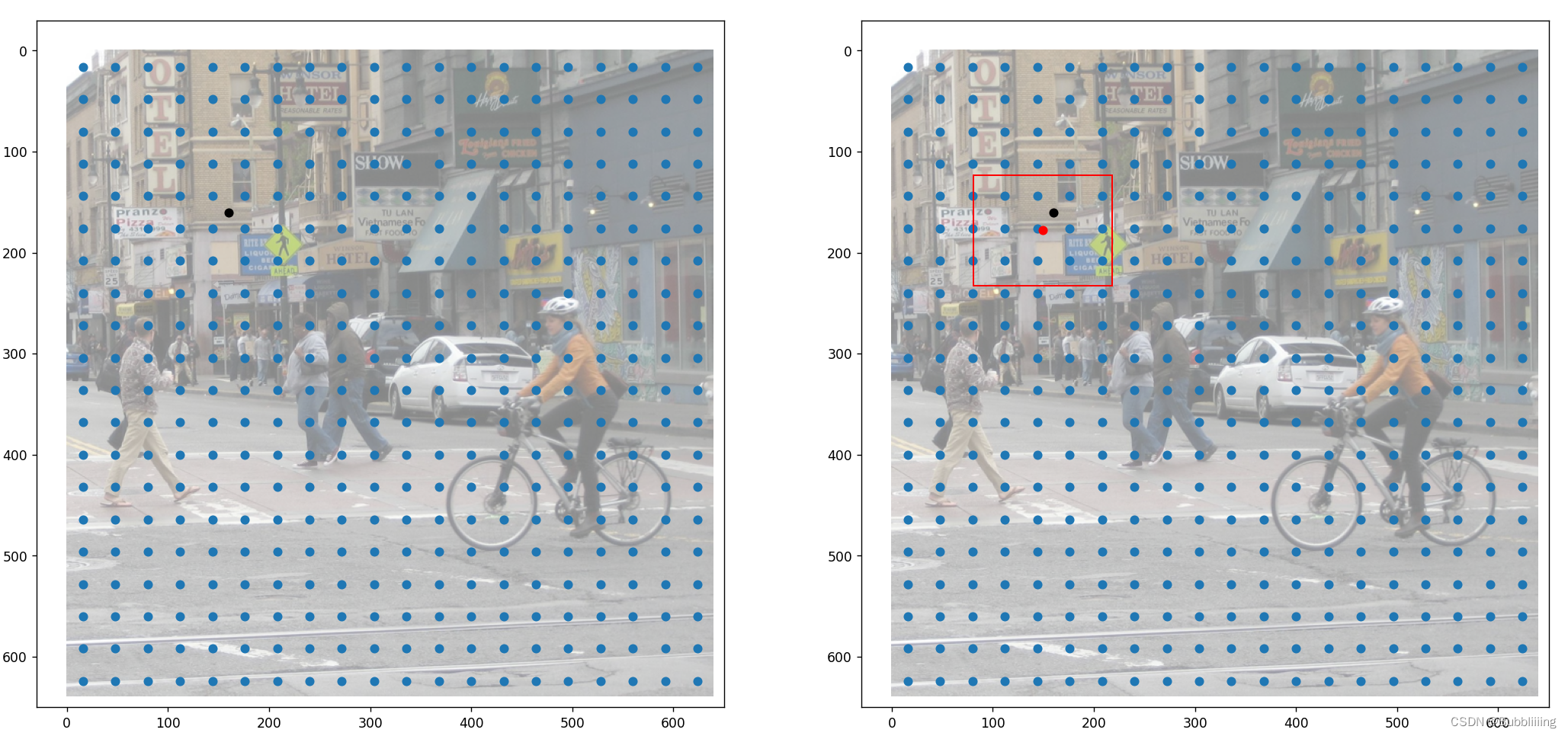
In addition to such decoding operations, there are also non-greatly suppressed operations that need to be performed to prevent the stacking of boxes of the same kind.

def dist2bbox(distance, anchor_points, xywh=True, dim=-1):
"""Transform distance(ltrb) to box(xywh or xyxy)."""
# Top left, bottom right
lt, rb  = torch.split(distance, 2, dim)
x1y1    = anchor_points - lt
x2y2    = anchor_points + rb
if xywh:
c_xy    = (x1y1 + x2y2) / 2
wh      = x2y2 - x1y1
return torch.cat((c_xy, wh), dim)  # xywh bbox
return torch.cat((x1y1, x2y2), dim)  # xyxy bbox
def decode_box(self, inputs):
# dbox  batch_size, 4, 8400
# cls   batch_size, 20, 8400
dbox, cls, origin_cls, anchors, strides = inputs
# Get center width and height coordinates
dbox    = dist2bbox(dbox, anchors.unsqueeze(0), xywh=True, dim=1) * strides
y       = torch.cat((dbox, cls.sigmoid()), 1).permute(0, 2, 1)
# Normalize to between 0 and 1 #
y[:, :, :4] = y[:, :, :4] / torch.Tensor([self.input_shape[1], self.input_shape[0], self.input_shape[1], self.input_shape[0]]).to(y.device)
return y

2. Score screening and non-great suppression

After obtaining the final prediction results it is also necessary toScore Sorting and Non-Great Suppression Screening。

Score Screeningjust likeFilter the prediction frames whose scores satisfy the CONFIDENCE confidence level.
non-tremendous suppressionjust likeFilter the boxes that have the highest score for belonging to the same species in a given area.

The process of score screening and non-great suppression can be summarized as follows:
1、Find out the picture in theBoxes with scores greater than the threshold functionThe In carrying out theScreening for scores right before filtering for overlapping boxes can drastically reduce the number of boxes.
2. ToType for cycling, the role of non-maximal inhibition isFilter out the boxes that have the highest score for belonging to the same species in a given area, looping over the kinds canhelps us to perform non-great suppression for each class separately.
3. Sort the category from largest to smallest based on score.
4. Take out the box with the largest score each time and calculate theits degree of overlap with all other prediction frames, and those with too much overlap are eliminated.

The results after score screening and non-great suppression can then be used to plot the prediction frames.

The figure below is after non-great suppression.

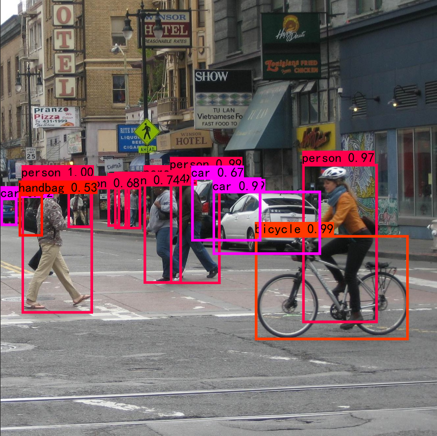
The figure below is without non-great suppression.

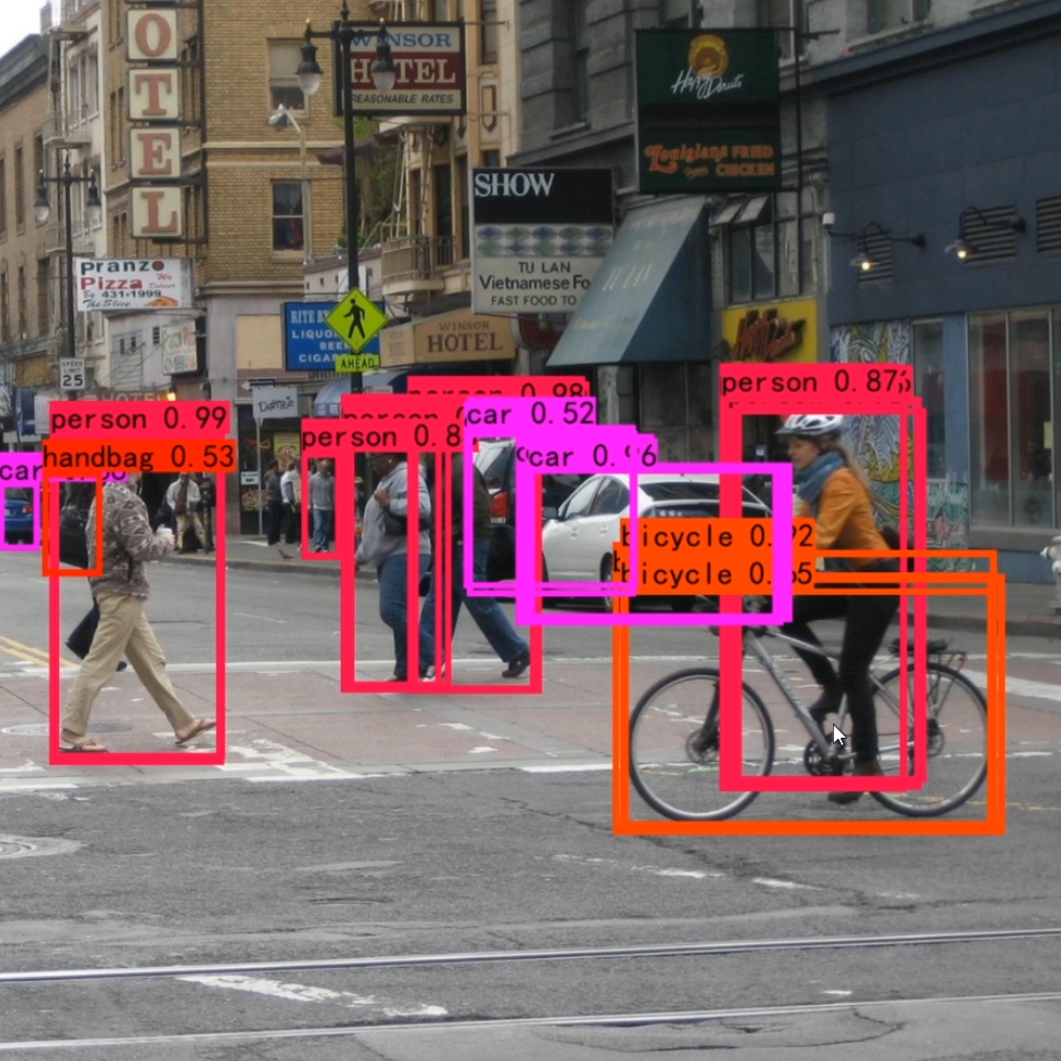
The implementation code is:

def non_max_suppression(self, prediction, num_classes, input_shape, image_shape, letterbox_image, conf_thres=0.5, nms_thres=0.4):
#----------------------------------------------------------#
# Convert the format of the prediction results to a top-left, bottom-right format.
#   prediction  [batch_size, num_anchors, 85]
#----------------------------------------------------------#
box_corner          = prediction.new(prediction.shape)
box_corner[:, :, 0] = prediction[:, :, 0] - prediction[:, :, 2] / 2
box_corner[:, :, 1] = prediction[:, :, 1] - prediction[:, :, 3] / 2
box_corner[:, :, 2] = prediction[:, :, 0] + prediction[:, :, 2] / 2
box_corner[:, :, 3] = prediction[:, :, 1] + prediction[:, :, 3] / 2
prediction[:, :, :4] = box_corner[:, :, :4]
output = [None for _ in range(len(prediction))]
for i, image_pred in enumerate(prediction):
#----------------------------------------------------------#
# Take max for the species prediction part.
# class_conf [num_anchors, 1] class_confidence
# class_pred [num_anchors, 1] type
#----------------------------------------------------------#
class_conf, class_pred = torch.max(image_pred[:, 4:4 + num_classes], 1, keepdim=True)
#----------------------------------------------------------#
# First round of screening using confidence levels
#----------------------------------------------------------#
conf_mask = (class_conf[:, 0] >= conf_thres).squeeze()
#----------------------------------------------------------#
# Screening of predictions based on confidence levels
#----------------------------------------------------------#
image_pred = image_pred[conf_mask]
class_conf = class_conf[conf_mask]
class_pred = class_pred[conf_mask]
if not image_pred.size(0):
continue
#-------------------------------------------------------------------------#
#   detections  [num_anchors, 6]
# 6 reads: x1, y1, x2, y2, class_conf, class_pred
#-------------------------------------------------------------------------#
detections = torch.cat((image_pred[:, :4], class_conf.float(), class_pred.float()), 1)
#------------------------------------------#
# Obtain all the categories included in the prediction results
#------------------------------------------#
unique_labels = detections[:, -1].cpu().unique()
if prediction.is_cuda:
unique_labels = unique_labels.cuda()
detections = detections.cuda()
for c in unique_labels:
#------------------------------------------#
# Obtain all predictions after screening for a particular type of score
#------------------------------------------#
detections_class = detections[detections[:, -1] == c]
#------------------------------------------#
# It's faster to use the official non-great suppression that comes with it!
# Sift through the boxes that have the highest scores for belonging to the same category in a given area
#------------------------------------------#
keep = nms(
detections_class[:, :4],
detections_class[:, 4],
nms_thres
)
max_detections = detections_class[keep]
# Sorted by confidence in the presence of the object
# _, conf_sort_index = torch.sort(detections_class[:, 4]*detections_class[:, 5], descending=True)
# detections_class = detections_class[conf_sort_index]
# # To perform non-extreme suppression #
# max_detections = []
# while detections_class.size(0):
# # Take out the highest confidence in this category and step down to determine if the overlap is greater than nms_thres, if so remove it
#     max_detections.append(detections_class[0].unsqueeze(0))
#     if len(detections_class) == 1:
#         break
#     ious = bbox_iou(max_detections[-1], detections_class[1:])
#     detections_class = detections_class[1:][ious < nms_thres]
# # Stacking
# max_detections = torch.cat(max_detections).data
# Add max detections to outputs
output[i] = max_detections if output[i] is None else torch.cat((output[i], max_detections))
if output[i] is not None:
output[i]           = output[i].cpu().numpy()
box_xy, box_wh      = (output[i][:, 0:2] + output[i][:, 2:4])/2, output[i][:, 2:4] - output[i][:, 0:2]
output[i][:, :4]    = self.yolo_correct_boxes(box_xy, box_wh, input_shape, image_shape, letterbox_image)
return output

IV. Training component

1. Calculate what is needed for the loss

Calculating the loss is actually a comparison between the predicted results of the network and the true results of the network.
Like the prediction result of the network, the loss of the network consists of two parts, the regression part, and the kind part. The regression part is the regression parameter judgment of the feature points, and the kind part is the kinds of objects contained in the feature points.

2. Matching process for positive samples

In YoloV8, the matching process of positive samples during training can be divided into three parts.

• Determine whether the feature point is in the real frame based on the spatial distance.
• Determine whether the feature point is in the topk in the real frame based on the cost function.
• Post-processing such as de-weighting.

what is calledpositive sample matchingThat’sFind which feature points are considered to have a corresponding true frame and be responsible for the prediction of this true frame。

a. Determine whether the feature point is in the prediction box or not

In the step, first determine whether the feature point is in the prediction frame or not based on the spatial distance.YoloV8 will do a coarse match for each true frame. Find which prior frames on which feature points can be responsible for the prediction of that true frame.

The code is based on the situation of the coordinates of the real frame with the feature points.Use the coordinates of the feature point to subtract the upper-left corner of the real frame, and use the lower-right corner of the real frame to subtract the coordinates of the feature point, and if these values are all greater than 0, then the feature point is inside the real frame.

def select_candidates_in_gts(xy_centers, gt_bboxes, eps=1e-9, roll_out=False):
"""select the positive anchor center in gt
Args:
xy_centers (Tensor): shape(h*w, 4)
gt_bboxes (Tensor): shape(b, n_boxes, 4)
Return:
(Tensor): shape(b, n_boxes, h*w)
"""
n_anchors       = xy_centers.shape[0]
bs, n_boxes, _  = gt_bboxes.shape
# Calculate the distance of each real box from the top left and bottom right of each anchors anchor point, and then find the min
# Ensure that the real box is near the anchor, enclosing it
if roll_out:
bbox_deltas = torch.empty((bs, n_boxes, n_anchors), device=gt_bboxes.device)
for b in range(bs):
lt, rb          = gt_bboxes[b].view(-1, 1, 4).chunk(2, 2)  # left-top, right-bottom
bbox_deltas[b]  = torch.cat((xy_centers[None] - lt, rb - xy_centers[None]),
dim=2).view(n_boxes, n_anchors, -1).amin(2).gt_(eps)
return bbox_deltas
else:
# The real box sits on top, right bottom left-top, right-bottom 
lt, rb      = gt_bboxes.view(-1, 1, 4).chunk(2, 2)  
# The distance of the real box from the top left and bottom right of each anchors anchor point
bbox_deltas = torch.cat((xy_centers[None] - lt, rb - xy_centers[None]), dim=2).view(bs, n_boxes, n_anchors, -1)
# return (bbox_deltas.min(3)[0] > eps).to(gt_bboxes.dtype)
return bbox_deltas.amin(3).gt_(eps)

b, determine whether the feature point is in the topk of the real frame

In YoloV8, we will calculate a Cost cost matrix that represents the cost relationship between each real frame and each feature point, the Cost cost matrix consists of two parts:
1. the degree of overlap between each real frame and the current feature point prediction frame;
2. the kind prediction accuracy of each real frame and the current feature point prediction frame;

Previous Yolo’s have done the cost function in a small way, and YoloV8 in a large way, which is not fundamentally different, the difference being whether or not you have subtracted by 1.
The higher the overlap between each real frame and the current feature point’s predicted frame, it means that this feature point has already tried to fit that real frame, and therefore it will have a higher Cost cost.

The higher the prediction accuracy of each real frame and the kind of frame predicted by the current feature point, it also means that this feature point has already tried to fit that real frame, so it will have a higher Cost cost.

The purpose of the Cost cost matrix is to adaptively find the true box that the current feature point should go to fit, the higher the overlap the more it needs to be fitted, the more accurate the classification the more it needs to be fitted, and the more it needs to be fitted within a certain radius.

YoloV8 does not use the idea of OTA, which matches a maximum of 13 feature points per true frame.

Therefore, the process of determining whether a feature point is in the topk of the real box is summarized as follows:
1, Calculate the degree of overlap between each real frame and each feature point prediction frame. Take the alpha index.
2.Calculate the prediction accuracy of the species for each real frame and each feature point prediction frame. Take the beta index.
3. sum to get Cost cost matrix.
4, the k points with the largest Cost are used as the positive samples for that real frame.

def get_pos_mask(self, pd_scores, pd_bboxes, gt_labels, gt_bboxes, anc_points, mask_gt):
# pd_scores bs, num_total_anchors, num_classes
# pd_bboxes bs, num_total_anchors, 4
# gt_labels bs, n_max_boxes, 1
# gt_bboxes bs, n_max_boxes, 4
# 
# align_metric is a calculated surrogate value, the probability that a given prior belongs to the class of a given real frame multiplied by the degree of overlap between a given prior and the real frame
# overlaps is the degree to which some a priori point overlaps the true frame
# align_metric, overlaps    bs, max_num_obj, 8400
align_metric, overlaps  = self.get_box_metrics(pd_scores, pd_bboxes, gt_labels, gt_bboxes)
# Positive sample anchors need to be satisfied simultaneously:
# 1. In the real box
# 2, is the most overlapping positive sample of the true frame topk
# 3. meet mask_gt
# get in_gts mask           b, max_num_obj, 8400
# Determine if the a priori point is in the true box
mask_in_gts             = select_candidates_in_gts(anc_points, gt_bboxes, roll_out=self.roll_out)
# get topk_metric mask      b, max_num_obj, 8400
# Determine if the anchor is in the topk of the real box
mask_topk               = self.select_topk_candidates(align_metric * mask_in_gts, topk_mask=mask_gt.repeat([1, 1, self.topk]).bool())
# merge all mask to a final mask, b, max_num_obj, h*w
# Real boxes exist, not padding
mask_pos                = mask_topk * mask_in_gts * mask_gt
return mask_pos, align_metric, overlaps
def get_box_metrics(self, pd_scores, pd_bboxes, gt_labels, gt_bboxes):
if self.roll_out:
align_metric    = torch.empty((self.bs, self.n_max_boxes, pd_scores.shape[1]), device=pd_scores.device)
overlaps        = torch.empty((self.bs, self.n_max_boxes, pd_scores.shape[1]), device=pd_scores.device)
ind_0           = torch.empty(self.n_max_boxes, dtype=torch.long)
for b in range(self.bs):
ind_0[:], ind_2 = b, gt_labels[b].squeeze(-1).long()
# Getting a score for belonging to this category
# bs, max_num_obj, 8400
bbox_scores     = pd_scores[ind_0, :, ind_2]  
# Calculate ciou for real and predicted frames
# bs, max_num_obj, 8400
overlaps[b]     = bbox_iou(gt_bboxes[b].unsqueeze(1), pd_bboxes[b].unsqueeze(0), xywh=False, CIoU=True).squeeze(2).clamp(0)
align_metric[b] = bbox_scores.pow(self.alpha) * overlaps[b].pow(self.beta)
else:
# 2, b, max_num_obj
ind = torch.zeros([2, self.bs, self.n_max_boxes], dtype=torch.long)       
# b, max_num_obj  
# [0] represents the first image of the
ind[0] = torch.arange(end=self.bs).view(-1, 1).repeat(1, self.n_max_boxes)  
# [1] Really what's the label #
ind[1] = gt_labels.long().squeeze(-1) 
# Getting a score for belonging to this category
# Fetch the probability that a priori point belongs to a class
# b, max_num_obj, 8400
bbox_scores = pd_scores[ind[0], :, ind[1]]  
# Calculate ciou for real and predicted frames
# bs, max_num_obj, 8400
overlaps        = bbox_iou(gt_bboxes.unsqueeze(2), pd_bboxes.unsqueeze(1), xywh=False, CIoU=True).squeeze(3).clamp(0)
align_metric    = bbox_scores.pow(self.alpha) * overlaps.pow(self.beta)
return align_metric, overlaps
def select_topk_candidates(self, metrics, largest=True, topk_mask=None):
"""
Args:
metrics     : (b, max_num_obj, h*w).
topk_mask   : (b, max_num_obj, topk) or None
"""
# 8400
num_anchors             = metrics.shape[-1] 
# b, max_num_obj, topk
topk_metrics, topk_idxs = torch.topk(metrics, self.topk, dim=-1, largest=largest)
if topk_mask is None:
topk_mask = (topk_metrics.max(-1, keepdim=True) > self.eps).tile([1, 1, self.topk])
# b, max_num_obj, topk
topk_idxs[~topk_mask] = 0
# b, max_num_obj, topk, 8400 -> b, max_num_obj, 8400
# This step gets is_in_topk as b, max_num_obj, 8400
# represents the top k a priori points corresponding to each true frame
if self.roll_out:
is_in_topk = torch.empty(metrics.shape, dtype=torch.long, device=metrics.device)
for b in range(len(topk_idxs)):
is_in_topk[b] = F.one_hot(topk_idxs[b], num_anchors).sum(-2)
else:
is_in_topk = F.one_hot(topk_idxs, num_anchors).sum(-2)
# Determine if the anchor is in the topk of the real box
is_in_topk = torch.where(is_in_topk > 1, 0, is_in_topk)
return is_in_topk.to(metrics.dtype)

c. Post-processing such as de-weighting

In the above process, there will be cases where the topk feature points of multiple real boxes are the same feature point. At this point we need to reverse the operation to find which real frame is the most suitable for this current feature point.

The way to determine which truth box is the best fit for this current feature point here is relatively simple.By determining how much each true frame overlaps with each predicted frame it is possible toThe greater the degree of overlap, the better the fit.

def select_highest_overlaps(mask_pos, overlaps, n_max_boxes):
"""if an anchor box is assigned to multiple gts,
the one with the highest iou will be selected.
Args:
mask_pos (Tensor): shape(b, n_max_boxes, h*w)
overlaps (Tensor): shape(b, n_max_boxes, h*w)
Return:
target_gt_idx (Tensor): shape(b, h*w)
fg_mask (Tensor): shape(b, h*w)
mask_pos (Tensor): shape(b, n_max_boxes, h*w)
"""
# b, n_max_boxes, 8400 -> b, 8400
fg_mask = mask_pos.sum(-2)
# If there is an anchor assigned to predict multiple true boxes
if fg_mask.max() > 1:  
# b, n_max_boxes, 8400
mask_multi_gts      = (fg_mask.unsqueeze(1) > 1).repeat([1, n_max_boxes, 1])  
# If there is an anchor assigned to predict multiple true boxes，首先计算这个anchor最重合的真实框
# And then do a onehot #
# b, 8400
max_overlaps_idx    = overlaps.argmax(1)  
# b, 8400, n_max_boxes
is_max_overlaps     = F.one_hot(max_overlaps_idx, n_max_boxes)  
# b, n_max_boxes, 8400
is_max_overlaps     = is_max_overlaps.permute(0, 2, 1).to(overlaps.dtype)  
# b, n_max_boxes, 8400
mask_pos            = torch.where(mask_multi_gts, is_max_overlaps, mask_pos) 
fg_mask             = mask_pos.sum(-2)
# Find out which gt each anchor fits into
target_gt_idx = mask_pos.argmax(-2)  # (b, h*w)
return target_gt_idx, fg_mask, mask_pos

3. Calculate Loss

As can be seen from the first part, the loss of YoloV8 consists of two parts:
1, the regression part, from the previous part, we can know the correspondence between each real frame and each prediction frame, and we can find the corresponding feature points through the prediction frame. Because YoloV8 uses DFL to make the final regression prediction, we need to add DFL loss in the regression part, the regression loss of YoloV8 is composed of iou loss and DFL loss.

• The iou loss component is relatively simple, and can be achieved directly by calculating the degree of overlap between the predicted frame and the true frame and using the 1-overlap degree.
• The DFL loss, on the other hand, goes to the regression loss in a probabilistic way and therefore uses the cross entropy
  The DFL sets the regression target as a categorical target, in the case of the x-coordinate of the point in the upper-left corner of the real box, which will not normally lie on a specific grid point, when its coordinates will not be integers (The computational loss is not relative to the real map, but to the mesh map for each feature layer）。
  Assuming that the x-coordinate of the real box is 7.9, then it is closer to 8 and farther from 7. We can then use the two cross-entropies in this way, thePrediction results with 7 seek cross entropy and give lower weights, prediction results with 8 seek cross entropy and give higher weights。

(8-7.9) * cross_entropy(pred_dist, 7)
+
(7.9-7) * cross_entropy(pred_dist, 8)

2. Kind part, from the previous part, we can know the correspondence between each real frame and each prediction frame, and we can find the corresponding feature point through the prediction frame. Take out the prediction result of the kind of the a priori box, calculate the cross-entropy loss according to the kind of the real box and the prediction result of the kind of the a priori box, as the Loss composition of the kind part.

The calculation part of the loss of species, however, the label is not 1 at this point, but is calculated by the degree of overlap of theBy multiplying the degree of overlap between the predicted frame and the real frame by the cost function and dividing by the maximum surrogate value corresponding to this real frame。

class BboxLoss(nn.Module):
def __init__(self, reg_max=16, use_dfl=False):
super().__init__()
self.reg_max = reg_max
self.use_dfl = use_dfl
def forward(self, pred_dist, pred_bboxes, anchor_points, target_bboxes, target_scores, target_scores_sum, fg_mask):
# Calculate IOU losses
# weight represents the confidence level that the labels in the loss should have, with 0 being the smallest and 1 being the largest
weight      = torch.masked_select(target_scores.sum(-1), fg_mask).unsqueeze(-1)
# Calculate the degree of overlap between the predicted and real frames
iou         = bbox_iou(pred_bboxes[fg_mask], target_bboxes[fg_mask], xywh=False, CIoU=True)
# Then 1- degree of overlap, multiply by the confidence level it should have, sum and average.
loss_iou    = ((1.0 - iou) * weight).sum() / target_scores_sum
# Calculate DFL losses
if self.use_dfl:
target_ltrb = bbox2dist(anchor_points, target_bboxes, self.reg_max)
loss_dfl = self._df_loss(pred_dist[fg_mask].view(-1, self.reg_max + 1), target_ltrb[fg_mask]) * weight
loss_dfl = loss_dfl.sum() / target_scores_sum
else:
loss_dfl = torch.tensor(0.0).to(pred_dist.device)
return loss_iou, loss_dfl
@staticmethod
def _df_loss(pred_dist, target):
# Return sum of left and right DFL losses
# Distribution Focal Loss (DFL) proposed in Generalized Focal Loss https://ieeexplore.ieee.org/document/9792391
tl = target.long()  # target left
tr = tl + 1  # target right
wl = tr - target  # weight left
wr = 1 - wl  # weight right
# A point is generally not at an anchor point, it is generally xx.xx. If you are going to use a DFL, it's unlikely that a direct cross_entropy will be fitted
# So think of it as the distance from the top left anchor to the bottom right anchor relative to xx.xx If the distance from the bottom right anchor is small, the wl is small and the top left loss is small
# If distance from top left anchor is small, wr is small, bottom right loss is small
return (F.cross_entropy(pred_dist, tl.view(-1), reduction="none").view(tl.shape) * wl +
F.cross_entropy(pred_dist, tr.view(-1), reduction="none").view(tl.shape) * wr).mean(-1, keepdim=True)
def xywh2xyxy(x):
"""
Convert bounding box coordinates from (x, y, width, height) format to (x1, y1, x2, y2) format where (x1, y1) is the
top-left corner and (x2, y2) is the bottom-right corner.
Args:
x (np.ndarray) or (torch.Tensor): The input bounding box coordinates in (x, y, width, height) format.
Returns:
y (np.ndarray) or (torch.Tensor): The bounding box coordinates in (x1, y1, x2, y2) format.
"""
y = x.clone() if isinstance(x, torch.Tensor) else np.copy(x)
y[..., 0] = x[..., 0] - x[..., 2] / 2  # top left x
y[..., 1] = x[..., 1] - x[..., 3] / 2  # top left y
y[..., 2] = x[..., 0] + x[..., 2] / 2  # bottom right x
y[..., 3] = x[..., 1] + x[..., 3] / 2  # bottom right y
return y
# Criterion class for computing training losses
class Loss:
def __init__(self, model): 
self.bce    = nn.BCEWithLogitsLoss(reduction='none')
self.stride = model.stride  # model strides
self.nc     = model.num_classes  # number of classes
self.no     = model.no
self.reg_max = model.reg_max
self.use_dfl = model.reg_max > 1
roll_out_thr = 64
self.assigner = TaskAlignedAssigner(topk=10,
num_classes=self.nc,
alpha=0.5,
beta=6.0,
roll_out_thr=roll_out_thr)
self.bbox_loss  = BboxLoss(model.reg_max - 1, use_dfl=self.use_dfl)
self.proj       = torch.arange(model.reg_max, dtype=torch.float)
def preprocess(self, targets, batch_size, scale_tensor):
if targets.shape[0] == 0:
out = torch.zeros(batch_size, 0, 5, device=targets.device)
else:
# Getting an image index
i           = targets[:, 0]  
_, counts   = i.unique(return_counts=True)
out         = torch.zeros(batch_size, counts.max(), 5, device=targets.device)
# Loop over the batch and assign a value
for j in range(batch_size):
matches = i == j
n = matches.sum()
if n:
out[j, :n] = targets[matches, 1:]
# Zoom to original image size.
out[..., 1:5] = xywh2xyxy(out[..., 1:5].mul_(scale_tensor))
return out
def bbox_decode(self, anchor_points, pred_dist):
if self.use_dfl:
# batch, anchors, channels
b, a, c     = pred_dist.shape  
# DFL decoding
pred_dist   = pred_dist.view(b, a, 4, c // 4).softmax(3).matmul(self.proj.to(pred_dist.device).type(pred_dist.dtype))
# pred_dist = pred_dist.view(b, a, c // 4, 4).transpose(2,3).softmax(3).matmul(self.proj.type(pred_dist.dtype))
# pred_dist = (pred_dist.view(b, a, c // 4, 4).softmax(2) * self.proj.type(pred_dist.dtype).view(1, 1, -1, 1)).sum(2)
# Then decode to get the prediction frame
return dist2bbox(pred_dist, anchor_points, xywh=False)
def __call__(self, preds, batch):
# Get the device used
device  = preds[1].device
# box, cls, dfl 3-part loss
loss    = torch.zeros(3, device=device)  
# Obtaining features and segmenting them
feats   = preds[2] if isinstance(preds, tuple) else preds
pred_distri, pred_scores = torch.cat([xi.view(feats[0].shape[0], self.no, -1) for xi in feats], 2).split((self.reg_max * 4, self.nc), 1)
# bs, num_classes + self.reg_max * 4 , 8400 =>  cls bs, num_classes, 8400; 
#                                               box bs, self.reg_max * 4, 8400
pred_scores = pred_scores.permute(0, 2, 1).contiguous()
pred_distri = pred_distri.permute(0, 2, 1).contiguous()
# Get batch size and dtype
dtype       = pred_scores.dtype
batch_size  = pred_scores.shape[0]
# Get input image size
imgsz       = torch.tensor(feats[0].shape[2:], device=device, dtype=dtype) * self.stride[0]  
# Get the tensor corresponding to the anchors points and step size
anchor_points, stride_tensor = make_anchors(feats, self.stride, 0.5)
# Make a matrix of what's in a batch #
# 0 is the first image that belongs to
# 1 for type
# 2: are the coordinates of the box
targets                 = torch.cat((batch[:, 0].view(-1, 1), batch[:, 1].view(-1, 1), batch[:, 2:]), 1)
# First do the initial processing, padding the incoming gt to the maximum amount and scaling the coordinates of the frame
# bs, max_boxes_num, 5
targets                 = self.preprocess(targets.to(device), batch_size, scale_tensor=imgsz[[1, 0, 1, 0]])
# bs, max_boxes_num, 5 => bs, max_boxes_num, 1 ; bs, max_boxes_num, 4
gt_labels, gt_bboxes    = targets.split((1, 4), 2)  # cls, xyxy
# Find out which boxes are targeted and which are populated
# bs, max_boxes_num
mask_gt                 = gt_bboxes.sum(2, keepdim=True).gt_(0)
# pboxes
# Decode the prediction results to obtain a prediction frame
# bs, 8400, 4
pred_bboxes             = self.bbox_decode(anchor_points, pred_distri)  # xyxy, (b, h*w, 4)
# Assignment of prediction frames to real frames
# target_bboxes     bs, 8400, 4
# target_scores     bs, 8400, 80
# fg_mask           bs, 8400
_, target_bboxes, target_scores, fg_mask, _ = self.assigner(
pred_scores.detach().sigmoid(), (pred_bboxes.detach() * stride_tensor).type(gt_bboxes.dtype),
anchor_points * stride_tensor, gt_labels, gt_bboxes, mask_gt
)
target_bboxes       /= stride_tensor
target_scores_sum   = max(target_scores.sum(), 1)
# Calculated categorized losses
# loss[1] = self.varifocal_loss(pred_scores, target_scores, target_labels) / target_scores_sum  # VFL way
loss[1] = self.bce(pred_scores, target_scores.to(dtype)).sum() / target_scores_sum  # BCE
# Calculate bbox losses
if fg_mask.sum():
loss[0], loss[2] = self.bbox_loss(pred_distri, pred_bboxes, anchor_points, target_bboxes, target_scores,
target_scores_sum, fg_mask)
loss[0] *= 7.5  # box gain
loss[1] *= 0.5  # cls gain
loss[2] *= 1.5  # dfl gain
return loss.sum() # loss(box, cls, dfl) # * batch_size

Train your own YoloV8 model

First, go to Github and download the corresponding repository, after downloading, unzip it using decompression software, and then open the folder with programming software.
Note that the root directory opened must be correct, otherwise the code will not run if the relative directory is not correct.
Be sure to note that the root directory after opening is the directory where the files are stored.

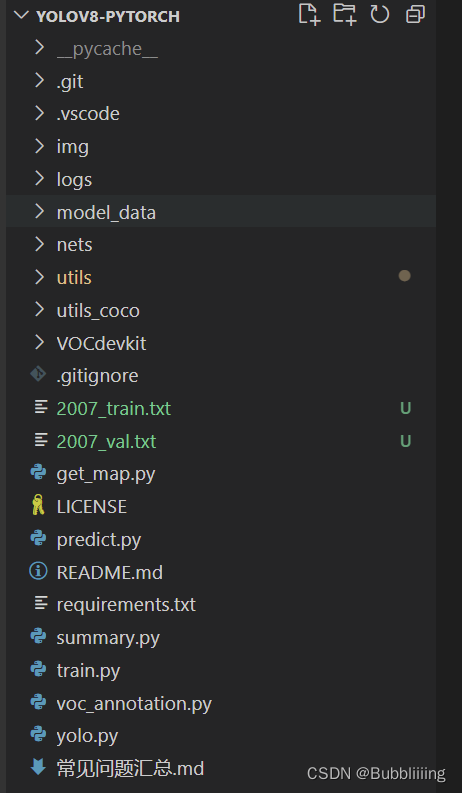
I. Preparation of data sets

This paper uses VOC format for training, you need to make your own dataset before training, if you don’t have your own dataset, you can download the VOC12+07 dataset through Github connection to try it out.
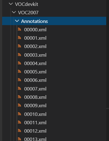
Place the label file in the VOCdevkit folder in the VOC2007 folder under Annotation before training.

Place the image files in JPEGImages in the VOC2007 folder under the VOCdevkit folder before training.

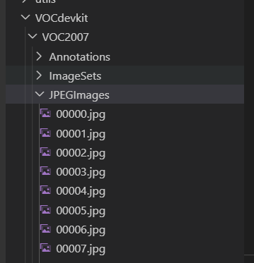
At this point the placement of the data set is complete.

II. Processing of data sets

After completing the placement of the dataset, we need to take the next step in processing the dataset with the aim of obtaining 2007_train.txt for training as well as 2007_val.txt, which requires the use of voc_annotation.py in the root directory.

Inside voc_annotation.py there are some parameters to set.
are annotation_mode, classes_path, trainval_percent, train_percent, and VOCdevkit_path, and for the first training, only classes_path can be modified.

'''
annotation_mode is used to specify the runtime calculations for this file
annotation_mode is 0 for the whole labeling process, including obtaining the txt inside VOCdevkit/VOC2007/ImageSets and 2007_train.txt and 2007_val.txt for training.
annotation_mode is 1 to get the txt in VOCdevkit/VOC2007/ImageSets.
The annotation_mode of 2 represents the acquisition of 2007_train.txt, 2007_val.txt for training purposes.
'''
annotation_mode     = 0
'''
Must be modified to generate target information for 2007_train.txt, 2007_val.txt
Just be consistent with the classes_path used for training and prediction
If there is no target information in the generated 2007_train.txt
Then it's because the classes aren't set correctly.
Only valid when annotation_mode is 0 and 2.
'''
classes_path        = 'model_data/voc_classes.txt'
'''
trainval_percent is used to specify the ratio of (training set + validation set) to test set, by default (training set + validation set):test set = 9:1
train_percent is used to specify the ratio of training set to validation set in (training set + validation set), by default training set:validation set = 9:1
Only valid when annotation_mode is 0 and 1.
'''
trainval_percent    = 0.9
train_percent       = 0.9
'''
Points to the folder where the VOC dataset is located
Default pointing to the VOC dataset in the root directory
'''
VOCdevkit_path  = 'VOCdevkit'

The classes_path is used to point to the txt corresponding to the detected class, in the case of the voc dataset, we use the txt as:

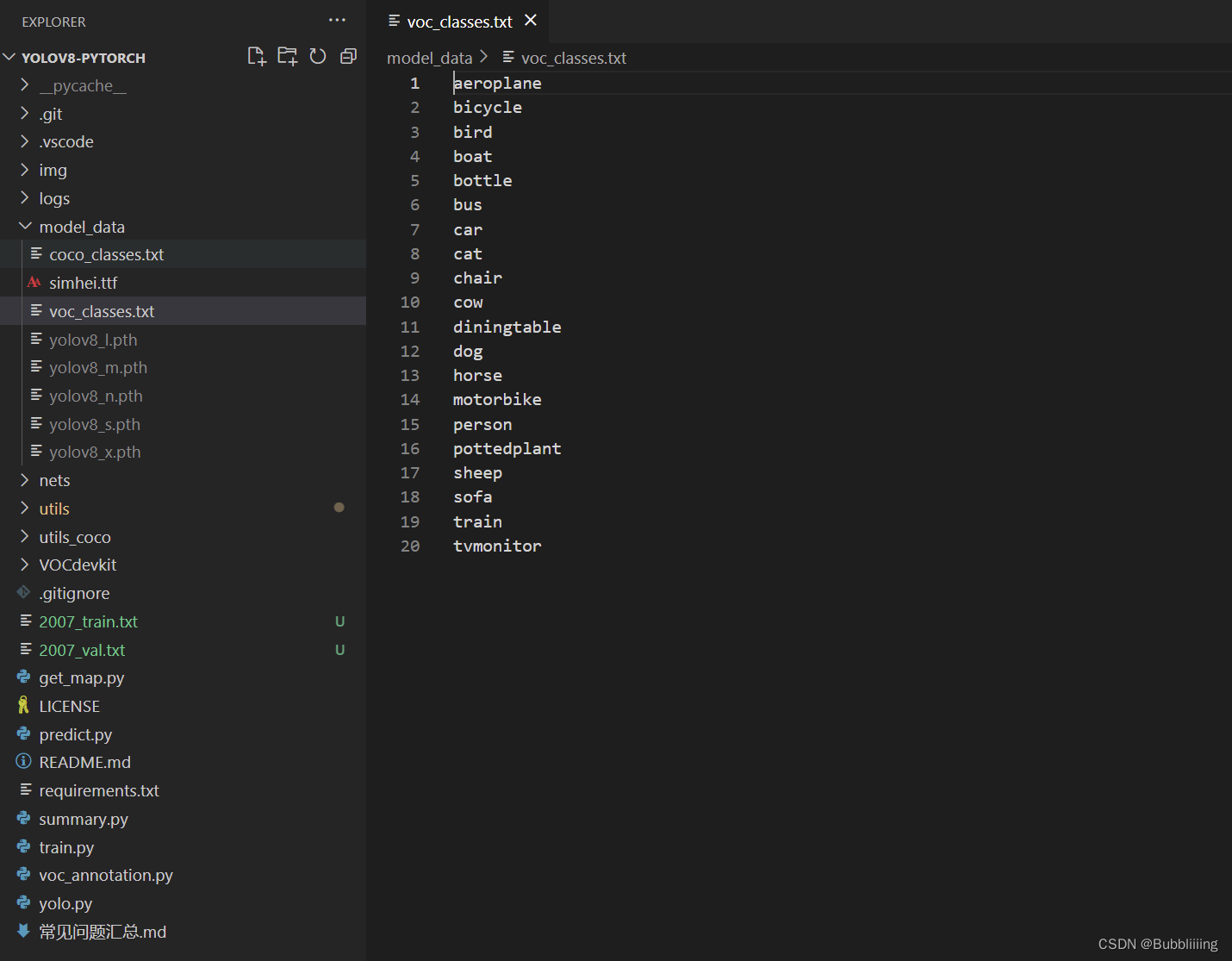
When training your own dataset, you can create a cls_classes.txt by yourself, in which you write the classes you need to distinguish.

III. Starting network training

With voc_annotation.py we have generated 2007_train.txt as well as 2007_val.txt and at this point we can start training.
There are more parameters for training, so you can read the comments carefully after downloading the library, the most important part of which remains the classes_path in train.py.

The classes_path is used to point to the txt corresponding to the detection class, which is the same as the txt inside voc_annotation.py! The dataset for training yourself has to be modified!

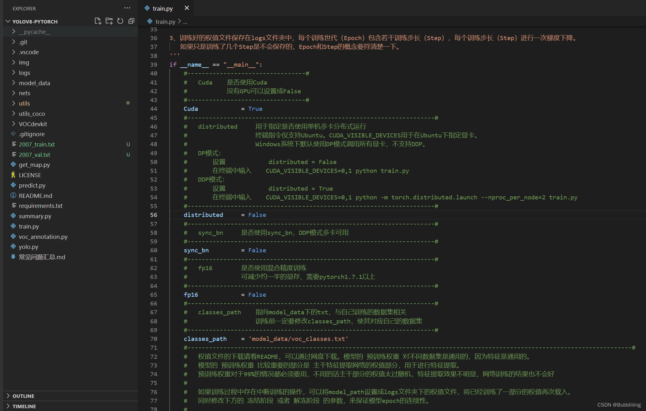
After modifying the classes_path you can run train.py to start training, after training multiple epochs the weights are generated in the logs folder.
The other parameters work as follows:

#---------------------------------#
# Cuda Whether to use Cuda
# No GPU can be set to False
#---------------------------------#
Cuda            = True
#---------------------------------------------------------------------#
# distributed Used to specify whether or not to use single-computer, multi-card distributed operation
# Terminal commands are only supported for Ubuntu. CUDA_VISIBLE_DEVICES is used to specify the graphics card under Ubuntu.
# Windows systems use DP mode to invoke all graphics cards by default, DDP is not supported.
# DP mode:
# Set distributed = False
# Type CUDA_VISIBLE_DEVICES=0,1 in the terminal python train.py
# DDP mode:
# Set distributed = True
# In the terminal, enter CUDA_VISIBLE_DEVICES=0,1 python -m torch.distributed.launch --nproc_per_node=2 train.py
#---------------------------------------------------------------------#
distributed     = False
#---------------------------------------------------------------------#
# sync_bn Whether to use sync_bn, DDP mode multi-card available
#---------------------------------------------------------------------#
sync_bn         = False
#---------------------------------------------------------------------#
# fp16 whether to train with mixed precision
# Reduces video memory by about half, requires pytorch 1.7.1+.
#---------------------------------------------------------------------#
fp16            = False
#---------------------------------------------------------------------#
# classes_path points to a txt under model_data, related to your own training dataset 
# Be sure to modify the classes_path before training so that it corresponds to your own dataset
#---------------------------------------------------------------------#
classes_path    = 'model_data/voc_classes.txt'
#----------------------------------------------------------------------------------------------------------------------------#
# See the README for the weights file, which can be downloaded via the netbook. Pre-training weights for the model are common to different datasets because the features are common.
# Pre-training weights for the model The more important part is the weights part of the backbone feature extraction network, which is used for feature extraction.
# Pre-training weights are necessary for 99% of the cases, if not, the weights in the main part are too random, the feature extraction is not effective, and the results of the network training will not be good
#
# If there is an interruption of training during the training process, you can set the model_path to the weights file in the logs folder to reload the weights that have already been partially trained.
# Also modify the parameters of the Freeze or Thaw phases below to ensure the continuity of the model epoch.
#   
# Do not load weights for the whole model when model_path = ''.
#
# Here the weights for the whole model are used, so they are loaded in train.py.
# If you want the model to start training from 0, set model_path = '' and Freeze_Train = Fasle below, at which point it starts training from 0 and there is no process of freezing the backbone.
#   
# In general, the network will train poorly from 0 because the weights are too random and the feature extraction is not effective, so it is very, very, very much not recommended that you start training from 0!
# There are two options for training from 0:
# 1, thanks to the powerful data enhancement capability of Mosaic data enhancement method, with UnFreeze_Epoch set to larger (300 and above), larger batch (16 and above), and more data (10,000 and above).
# It is possible to set mosaic=True and just randomly initialize the parameters to start training, but the results obtained are still not as good as with pre-training. (This can be done for large datasets like COCO)
# 2. Understand the imagenet dataset, first train the classification model to obtain the weights of the backbone part of the network, the backbone part of the classification model is common to this model, based on which training is carried out.
#----------------------------------------------------------------------------------------------------------------------------#
model_path      = 'model_data/yolov8_s.pth'
#------------------------------------------------------#
# input_shape The input shape size, must be a multiple of 32.
#------------------------------------------------------#
input_shape     = [640, 640]
#------------------------------------------------------#
# The version of yolov8 used by phi.
# n : corresponds to yolov8_n
# s : corresponds to yolov8_s
# m : corresponds to yolov8_m
# l : corresponds to yolov8_l
# x : corresponds to yolov8_x
#------------------------------------------------------#
phi             = 's'
#----------------------------------------------------------------------------------------------------------------------------#
# pretrained Whether to use the pretrained weights of the backbone network, which are used here and therefore loaded during model construction.
# If model_path is set, the weights of the trunk do not need to be loaded and the pretrained values are meaningless.
# If model_path is not set, pretrained = True, at which point only the trunk is loaded to start training.
# If model_path is not set, pretrained = False, Freeze_Train = Fasle, at which point training starts at 0 and there is no process of freezing the backbone.
#----------------------------------------------------------------------------------------------------------------------------#
pretrained      = False
#------------------------------------------------------------------#
# mosaic mosaic data enhancement.
# mosaic_prob What is the probability that each STEP will use mosaic data augmentation, default 50%.
#
# mixup Whether or not to use mixup data enhancement, only valid if mosaic=True.
# will only mixup mosaic enhanced images.
# mixup_prob What is the probability of using mixup data enhancement after mosaic, default 50%.
# The total mixup probability is mosaic_prob * mixup_prob.
#
# special_aug_ratio Refer to YoloX, since Mosaic generates training images that are far from the true distribution of natural images.
# When mosaic=True, this code turns on mosaic in the special_aug_ratio range.
# Defaults to the first 70% of epochs, 100 generations will open 70 generations.
#------------------------------------------------------------------#
mosaic              = True
mosaic_prob         = 0.5
mixup               = True
mixup_prob          = 0.5
special_aug_ratio   = 0.7
#------------------------------------------------------------------#
# label_smoothing Label smoothing. Generally 0.01 or less. E.g. 0.01, 0.005.
#------------------------------------------------------------------#
label_smoothing     = 0
#----------------------------------------------------------------------------------------------------------------------------#
# Training is divided into two phases, the freeze phase and the unfreeze phase. The freezing phase is set up to fulfill the training needs of students whose machines are underperforming.
# Freeze_Train requires less video memory, and in the case of a very poor graphics card, you can set Freeze_Epoch equal to UnFreeze_Epoch, Freeze_Train = True, and then just do freeze training.
#      
# A number of parameter setting suggestions are provided here, and you trainers have the flexibility to adjust them according to your needs:
# (i) Start training with pre-training weights for the entire model: 
#       Adam：
# Init_Epoch = 0, Freeze_Epoch = 50, UnFreeze_Epoch = 100, Freeze_Train = True, optimizer_type = 'adam', Init_lr = 1e-3, weight_decay = 0. (Freeze)
# Init_Epoch = 0, UnFreeze_Epoch = 100, Freeze_Train = False, optimizer_type = 'adam', Init_lr = 1e-3, weight_decay = 0. (No freeze)
#       SGD：
# Init_Epoch = 0, Freeze_Epoch = 50, UnFreeze_Epoch = 300, Freeze_Train = True, optimizer_type = 'sgd', Init_lr = 1e-2, weight_decay = 5e-4. (Freeze)
# Init_Epoch = 0, UnFreeze_Epoch = 300, Freeze_Train = False, optimizer_type = 'sgd', Init_lr = 1e-2, weight_decay = 5e-4. (not frozen)
# Where: UnFreeze_Epoch can be adjusted between 100-300.
# (ii) Training from 0:
# Init_Epoch = 0, UnFreeze_Epoch >= 300, Unfreeze_batch_size >= 16, Freeze_Train = False (no freeze training)
# where UnFreeze_Epoch is as close to 300 as possible. optimizer_type = 'sgd', Init_lr = 1e-2, mosaic = True.
# (iii) batch_size setting:
# Within the acceptable range of the graphics card, bigger is better. Insufficient memory has nothing to do with the dataset size, please adjust the batch_size down if you are prompted with insufficient memory (OOM or CUDA out of memory).
# Influenced by the BatchNorm layer, batch_size is at least 2, not 1.
# Under normal circumstances Freeze_batch_size is recommended to be 1-2 times of Unfreeze_batch_size. It is not recommended to set the gap too large, as it is related to the automatic adjustment of the learning rate.
#----------------------------------------------------------------------------------------------------------------------------#
#------------------------------------------------------------------#
# Freeze phase training parameters
# At this point the backbone of the model is frozen and the feature extraction network is unchanged #
# Uses less video memory and only fine tunes the network
# Init_Epoch The current starting training generation of the model, which can have a value greater than Freeze_Epoch, as set:
#                       Init_Epoch = 60、Freeze_Epoch = 50、UnFreeze_Epoch = 100
# Will skip the freeze phase and start directly from generation 60 and adjust the corresponding learning rate.
# (to be used during breakpoints)
# Freeze_Epoch model freeze trained Freeze_Epoch
# (disabled when Freeze_Train=False)
# Freeze_batch_size batch_size for model freeze training
# (disabled when Freeze_Train=False)
#------------------------------------------------------------------#
Init_Epoch          = 0
Freeze_Epoch        = 50
Freeze_batch_size   = 32
#------------------------------------------------------------------#
# Training parameters for thawing phase
# At this point the backbone of the model is not frozen anymore and the feature extraction network will change #
# Larger amount of video memory used, all parameters of the network change
# Total epochs trained for the UnFreeze_Epoch model
# SGD takes longer to converge, so set larger UnFreeze_Epoch
# Adam can use the relatively small UnFreeze_Epoch
# Unfreeze_batch_size batch_size of model after unfreezing
#------------------------------------------------------------------#
UnFreeze_Epoch      = 300
Unfreeze_batch_size = 16
#------------------------------------------------------------------#
# Freeze_Train whether or not to freeze training
# Defaults to freezing trunk training before unfreezing it.
#------------------------------------------------------------------#
Freeze_Train        = True
#------------------------------------------------------------------#
# Other training parameters: learning rate, optimizer, learning rate degradation related to
#------------------------------------------------------------------#
#------------------------------------------------------------------#
# Maximum learning rate for the Init_lr model
# Minimum learning rate for the Min_lr model, defaults to 0.01 of the maximum learning rate
#------------------------------------------------------------------#
Init_lr             = 1e-2
Min_lr              = Init_lr * 0.01
#------------------------------------------------------------------#
# optimizer_type the type of optimizer to use, optional adam, sgd
# It is recommended to set Init_lr=1e-3 when using the Adam optimizer.
# It is recommended to set Init_lr=1e-2 when using the SGD optimizer
# momentum The momentum parameter is used internally by the optimizer.
# weight_decay weight_decay to prevent overfitting
# adam causes weight_decay errors, it is recommended to set it to 0 when using adam.
#------------------------------------------------------------------#
optimizer_type      = "sgd"
momentum            = 0.937
weight_decay        = 5e-4
#------------------------------------------------------------------#
# lr_decay_type Learning rate descent method used, options are step, cos
#------------------------------------------------------------------#
lr_decay_type       = "cos"
#------------------------------------------------------------------#
# save_period how many epochs to save weights once
#------------------------------------------------------------------#
save_period         = 10
#------------------------------------------------------------------#
# save_dir Folder where permissions and log files are saved
#------------------------------------------------------------------#
save_dir            = 'logs'
#------------------------------------------------------------------#
# eval_flag Whether to evaluate at training time for the validation set
# The evaluation experience is better when the pycocotools library is installed.
# eval_period represents how many epochs to evaluate once, not recommended to evaluate frequently
# Evaluations are more time consuming and frequent evaluations can lead to very slow training
# The mAP obtained here will be different from the one obtained by get_map.py for two reasons:
# (i) The mAP obtained here is the mAP of the validation set.
# (ii) The assessment parameters here are set more conservatively in order to speed up the assessment.
#------------------------------------------------------------------#
eval_flag           = True
eval_period         = 10
#------------------------------------------------------------------#
# num_workers is used to set whether or not to use multiple threads to read the data
# Enabled will speed up data reads, but will use more memory
# Computers with less memory can be set to 2 or 0  
#------------------------------------------------------------------#
num_workers         = 4

IV. Prediction of training results

Two files are required for training result prediction, yolo.py and predict.py.
We first need to go to yolo.py and change model_path and classes_path, which must be changed.

model_path points to the trained weights file in the logs folder.
classes_path points to the txt corresponding to the detected class.

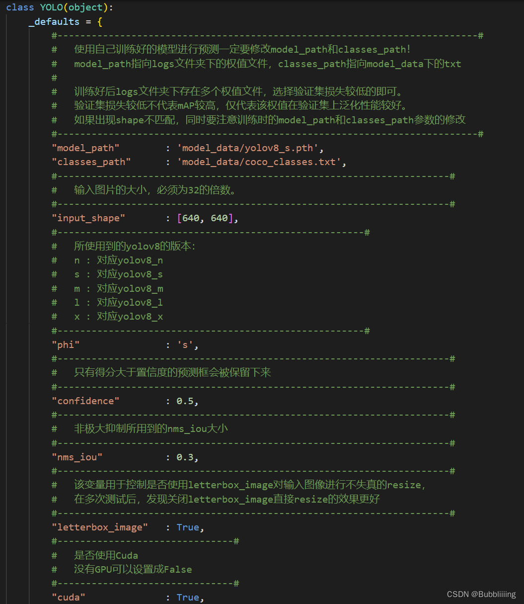
After completing the changes you can run predict.py to detect it. After running it, enter the path of the image to be detected.