🎉Author’s Profile:I am a graduate student in computer science, currently in my second year of study. Main research interests are in the direction of artificial intelligence and swarm intelligence algorithms. Currently familiar with python web crawler, machine learning, computer vision (OpenCV), swarm intelligence algorithms currently learning about deep learning.
📃Personal homepage:Fish that eats cats python personal homepage
🔎be in favor of:If you think the blogger’s article is not bad or you use it, you can follow the blogger free of charge, if three consecutive favorites support is even better! It is to give me the greatest support!
💛Abstract:
This column will be very detailed explanation related to computer vision OpenCV related knowledge that operation, very simple and easy to understand. This article mainly explains the relevant and computer vision related to the introduction of the content, about the image processing related to the simple operation, including reading images, display images and image-related theoretical knowledge.
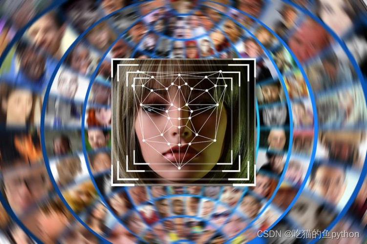
I. What is computer vision
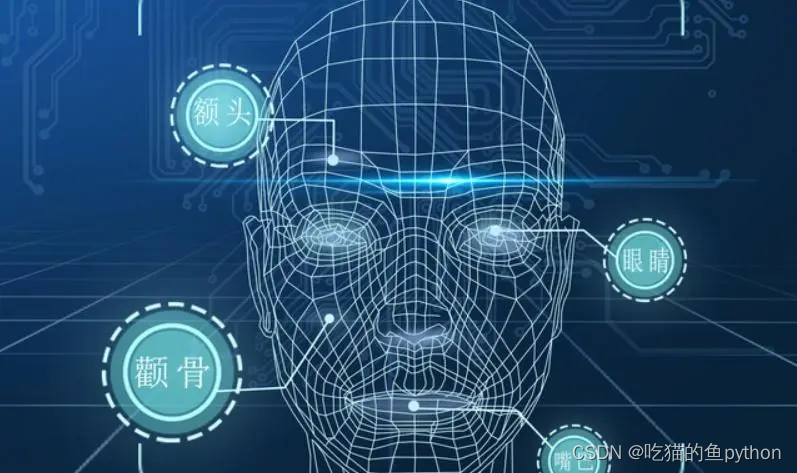
Computer vision is the science of how to make machines “see”, and furthermore, it refers to the use of cameras and computers instead of the human eye to identify, track, and measure the target of the machine vision, and further graphic processing, so that the computer processing to become more suitable for the human eye to observe or transmit to the instrument detection of the image. As a scientific discipline, computer vision studies the related theories and techniques in an attempt to build artificial intelligence systems that are capable of obtaining ‘information’ from images or multidimensional data. Information in this context is defined by Shannon as information that can be used to help make a ‘decision’. Since perception can be thought of as extracting information from sensory signals, computer vision can also be thought of as the science of how to make artificial systems ‘perceive’ from images or multidimensional data.
Vision is an important part of various application areas such asIn a variety of intelligent/autonomous systems in manufacturing, inspection, document analysis, medical diagnostics, and military applications.An integral part. Because of its importance, some advanced countries, such as the United States, have categorized research on computer vision as a major fundamental problem in science and engineering that has wide-ranging economic and scientific implications, the so-called grand challenge. The challenge of computer vision is to develop visual capabilities for computers and robots that are comparable to the human level. Machine vision requires graphical signals, texture and color modeling, geometric processing and reasoning, and object modeling. A capable vision system should tightly integrate all these processes.
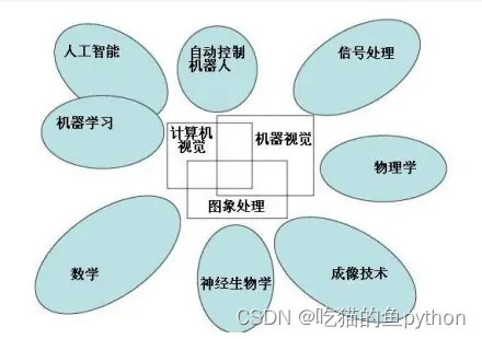
We are currently if the school students, for computer vision and machine learning related knowledge of learning is very useful, both for their own job prospects or related to the writing of the paper is very useful, and at present for the computer related knowledge has been designed to a variety of professional fields, including the medical field (computer vision to analyze the CT imaging), the field of electricity (using matlab (using matlab and related fields to draw diagrams), face recognition and license plate recognition, and so on. And there are those who want to do cross-discipline for computer can be and any field and carry on the cross without obstacles.
Since I am a man of science and technology is not good at language skills, language organization is not strong, so we will be wordy here today, the summary is that computer vision and machine learning and other things related to computers are particularly important!
II. Basic operation of image processing

First let’s look at a simple piece of computer vision related code:
import cv2
img=cv2.imread('path')#path refers to the relevant path of the image
cv2.imshow('Demo',img)
cv2.nameWindow('Demo')
cv2.waitKey(0)
cv2.destroyAllWindows()
This code then displays the image associated with img in your computer. Next we explain the operations associated with each step.
Image processing: reading in images
Related Functions: image=cv2.imread(file name related path [display control parameter])
Filename: the full path.
Among the parameters are:
cv.IMREAD_UNCHANGED : Indicates consistency with the original image.
cv.IMREAD_GRAYSCALE : Indicates that the original image is converted to a gray image.
cv.IMREAD_COLOR: Indicates that the original image is converted to a color image.
Example:
cv2.imread(‘d:\image.jpg’,cv.IMREAD_UNCHANGED)
Image processing: displaying images
Related functions: None=cv2.imshow(window name, image name)
Example: cv2.imshow(“demo”, image)
But in OpenCV we image display still have to add the relevant constraints:
retval=cv2.waitKey([delay])
If there is no such limitation, then the displayed image will flash and an error will occur.
where the delay parameter is included:
dealy=0, waits indefinitely for the image to be displayed until it is turned off. Also the default value for waitKey.
delay<0,wait for keyboard click to end the image display, that is, when we hit the keyboard, the image ends the display.
delay>0, wait for delay milliseconds to end the image display.
And finally we need to show the
cv2.destroyAllWindows()
Delete the image completely from memory.
Image processing: image saving
Related functions: retval=cv2.imwrite(file address, file name)
Example:
cv2.imwrite(‘D:\test.jpg’,img)
Saved img to path D:\test.jpg
III. Introductory Basics of Image Processing
Introduction to Image Imaging Principles
The first concept we need to engrave deeply and profoundly in our minds is:
| Pictures are made up of pixel dots. |
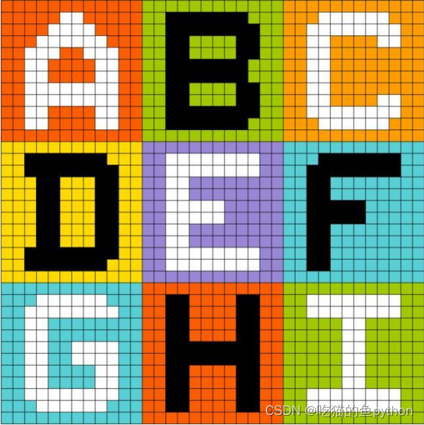
A little more vividly indicates that this is the case:
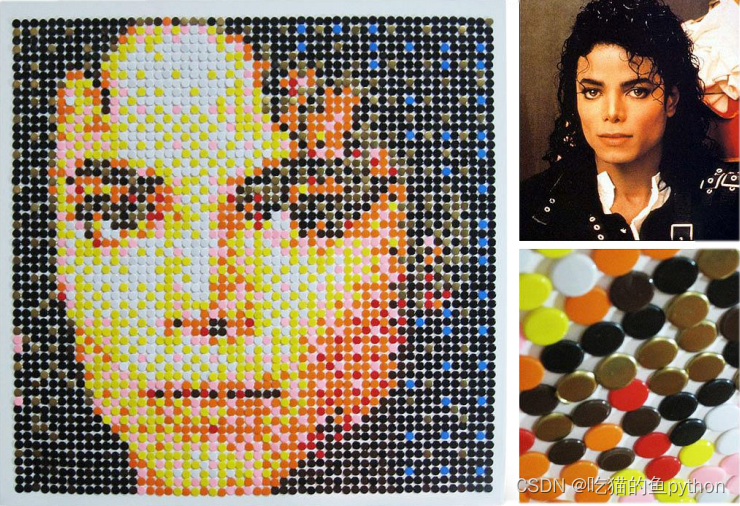
This perfectly demonstrates the imaging principle of a computer image, which is a patchwork of colored pixel dots.
image classification
Images are generally divided into three categories:
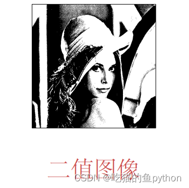
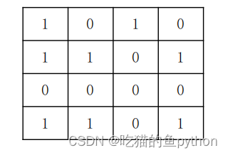
I. Binary Images
A binary image representation means that each pixel point consists of only 0 and 1. 0 means black and 1 means white, and here the black and white are pure black and pure white. So that’s what we see in the image. Let’s take the official website Lina as an example.
II. Gray-scale images
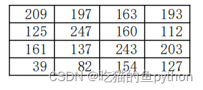
A grayscale image is an 8-bit bitmap. What does that mean? It means 00000001 all the way to 11111111, which is the binary representation. If it is expressed as our common decimal is 0-255, where 0 means pure black, 255 means pure white, in the middle is in pure black to pure white color. Let’s take Lena as an example.

Grayscale image a block of pixel points:
III. Color images (RGB)
All colors in a computer can be made up of R (red channel), G (green channel), and B (blue channel), where each channel is made up of 0-255 pixel colors. For example, R=234, G=252, and B=4 means yellow. The display is also yellow. So the color image consists of three sides, corresponding to R,G,B. Let’s take Lena as an example:

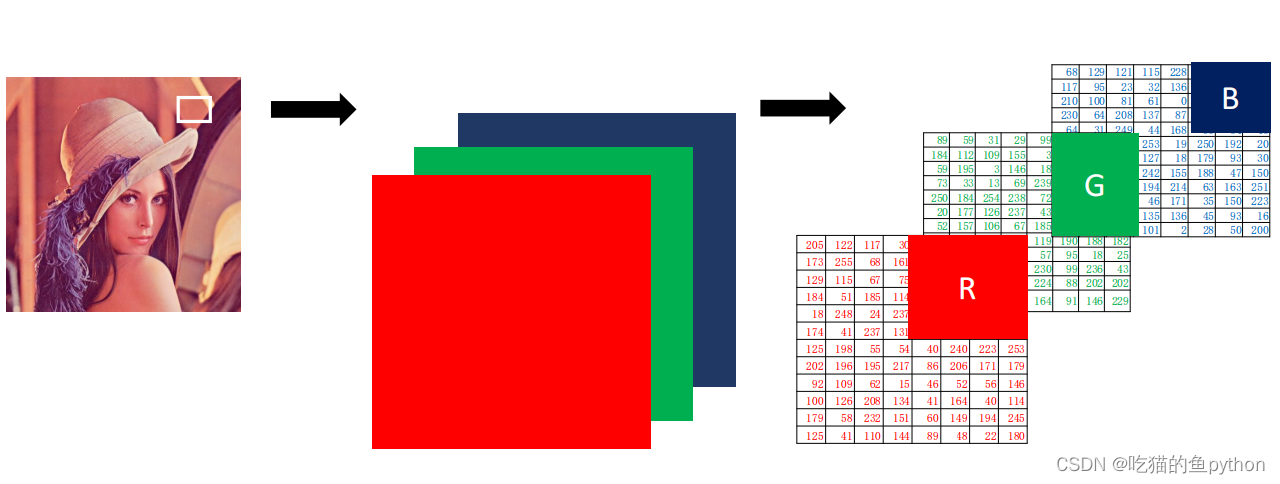
So we can know the order of complexity is: color image – grayscale image – binary image. So we are in the face project or license plate recognition project in the most commonly used operation is the color image into a gray-scale image, and then the gray-scale image into the simplest binary image.
IV. Pixel processing operations
Read Pixel
Related Functions: return value = image (positional parameter) Let’s start with a grayscale image and return the grayscale value:
p=img[88,142]
print§
Here we can return the grayscale value at the image coordinates [88, 142].
Then we take a color image as an example:
We know that a color image consists of the values of the three BGR channels. Then we need to return three values:
blue=img[78,125,0]
green=img[78,125,1]
red=img[78,125,2]
print(blue,green,red)
This way we return these three values.
Modify Pixel
Direct violent modification.
For a grayscale image, img[88, 99] = 255
For color images, the
img[88,99,0]=255
img][88,99,1]=255
img[88, 99, 2]=255 Here it can also be written as
img[88, 99]=[255, 255, 255] Equivalent to above.
Change multiple pixel points
For example, let’s still use a color image as an example:
i[100:150,100:150]=[255,255,255]
It also means that this interval between the image’s horizontal coordinates of 100 to 150 and vertical coordinates of 100 to 150 are all replaced with white.
Modifying pixel points with numpy in python
Read Pixel
Related function: return value = image.item (position parameter)
Let’s take a grayscale image as an example:
o=img,item(88,142)
print(o)
For color images we are still:
blue=img.item(88,142,0)
green=img.item(88,142,1)
red=img.item(88,142,2)
Then print(blue, green, red)
Modify Pixel
Image name.itemset (position, new value)
Let’s take a grayscale image as an example:
img.itemset((88,99),255)
For BGR images:
img.itemset((88,99,0),255)
img.itemset((88,99,1),255)
img.itemset((88,99,2),255)
import cv2
import numpy as np
i=cv2.imread('path',cv2.IMREAD_UNCHANGED)
print(i.item(100,100))
i.itemset((100,100),255)
print(i,item(100,100))
With this code we can see the pixel change.
The same is true for color images.
V. Getting Image Properties
shape
shape can get the shape of the image, the return value contains the number of rows, the number of columns, the number of channels of the tuple.
Gray scale image returns the number of rows and columns
The color image returns the number of rows, columns, and channels.
import cv2
img1=cv2.imread('grayscale image')
print(img1.shape)
image primitive order
size gets the number of pixels in the image.
Grayscale image: number of rowscolumns
Color images: number of linesNumber of columns * number of channels
Image Type
dtype returns the datatype of the image
import cv2
img=cv2.imread('image name')
print(img.dtype)
VI. Image ROI
ROI (region of interest) indicates region of interest
- Outline the area to be processed from the image being processed as a box, circle, ellipse, or irregular polygon.
- Various operators and functions can be used to find the ROI and proceed to the next step.
import cv2
import numpy as np
a=cv2.imread('path')
b=np.ones((101,101,3))
b=a[220:400,250:350]
a[0:101,0:101]=b
cv2.imshow('o',a)
cv2.waitKey()
cv2.destroyAllWindows()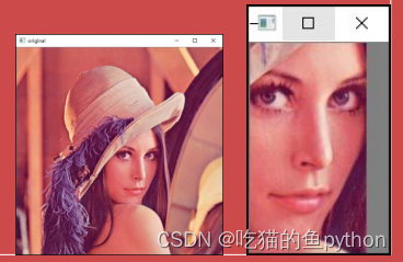
We can also add images of interest to other images.
VI. Splitting and merging of channels
broken up inseparate items
import cv2
img=cv2.imread('image name')
b = img[ : , : , 0 ]
g = img[ : , : , 1 ]
r = img[ : , : , 2 ]
We have functions in OpenCV that specialize in splitting channels:
cv2.split(img)
import cv2
import numpy as np
a=cv2.imread("image\lenacolor.png")
b,g,r=cv2.split(a)
cv2.imshow("B",b)
cv2.imshow("G",g)
cv2.imshow("R",r)
cv2.waitKey()
cv2.destroyAllWindows()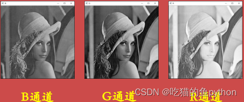
incorporation
import cv2
import numpy as np
a=cv2.imread("image\lenacolor.png")
b,g,r=cv2.split(a)
m=cv2.merge([b,g,r])
cv2.imshow("merge",m)
cv2.waitKey()
cv2.destroyAllWindows()
We merge the split image above to get the following result:

💐The article is suitable for all concerned to learn
🍀Don’t turn around immediately after reading this.
🌿Looking forward to the trifecta of following tiny bloggers plus favorites
🍃The little blogger is quick to return, and will give you an unexpected surprise.🍃
The bosses move small hands to give my little brother praise collection, more support is my power to update!
