Deep Learning – Convolutional Neural Network (CNN) Theory

Study period: 2022.04.10~2022.04.12

3. Convolutional neural network CNN

CNNs (Convolutional Neural Networks, ConvNets, Convolutional Neural Networks) are a type of neural network that is one of the best learning algorithms for understanding the content of an image and excels in tasks related to image segmentation, classification, detection and retrieval.

3.1 Concept of Convolutional Neural Networks

3.1.1 What is a CNN?

A CNN is a feedforward neural network with a convolutional structure thatconvolutional structureIt is possible to reduce the amount of memory occupied by the deep network, where three key operations – localizedexperience the wild、power sharing、ponding layer, effectively reducing the number of parameters of the network and alleviating the overfitting problem of the model.

Convolutional and pooling layers are generally taken a number of, using alternating setup of convolutional and pooling layers, i.e., a convolutional layer is connected to a pooling layer, and a pooling layer is connected to a convolutional layer after pooling, and so on. As each neuron of the output feature map in the convolutional layer is locally connected to its input, and the neuron input is obtained by weighting and summing the corresponding connection weights with the local inputs plus the bias value, this process is equivalent to the convolutional process, and the CNN is named after it.¹。

**Difference from ANN (Artificial Neural Networks):** Learned in the previous sectionMLP、BPIt is the ANN, which processes information by adjusting the internal neuron to neuron weighting relationships. And in CNN, its fully connected layer is is the MLP, except that a convolutional layer and a pooling layer are added in front of it.

CNN is mainly used in image recognition (computer vision, CV), applications include: image classification and retrieval, target localization detection, target segmentation, face recognition, bone recognition and tracking, as seen in MNIST handwritten data recognition, cat and dog fights, ImageNet LSVRC, etc., and can also be applied to natural language processing and speech recognition.

3.1.2 Why use CNNs?

In general, it is to solve two difficult problems: ① The amount of data to be processed for images is too large, resulting in high cost and low efficiency; ② It is difficult to retain the original features of images in the process of digitization, resulting in low accuracy of image processing.

• Reason 1: The image is large (disadvantage of fully connected BP neural networks)

Supplementary: Data structures for images

First thing to understand: a computer that stores pictures actually stores a$W\times H\times D$The array of ($W,H,D$(denoting width, height, and dimension, respectively; color images contain RGB 3D <red, green, and blue color channels>). Each number corresponds to the brightness of one pixel.

In a black and white image, we only need one matrix. Each matrix stores values between 0 and 255. This range is a compromise between the efficiency of storing image information (values within 256 can be expressed in exactly one byte) and the sensitivity of the human eye (we distinguish a finite number of gray values of the same color).

Current images used for computer vision problems are usually 224×224 or even larger, and if dealing with color images it is necessary to add another 3 color channels (RGB), i.e. 224x224x3.

If a BP neural network is constructed with 224x224x3=150528 pixel points to be processed, that is, 150528 input weights need to be processed, and if the hidden layer of this network has 1024 nodes (a typical hidden layer in this kind of network may have 1024 nodes), then, for the first hidden layer alone we have to train 150528×1024 = 1.5 billion weights. This is almost impossible to complete the training, let alone with larger images.

• Reason 2: Variable position

If you train a network to detect dogs, then you want it to detect dogs no matter which photo the image appears in.

If you build a BP neural network, you need to “flatten” the input image (i.e., turn the array into a column and feed it into the neural network for training). But this destroys the spatial information of the image. Imagine training a network that works well on an image of a dog, and then providing it with a slightly shifted version of the same image, where the network might react quite differently.

And, some related research shows that the human brain, in the process of understanding the information of the picture, does not observe the whole picture at the same time, but prefers to observe part of the features, and then according to the features to match, combine, and finally come up with the whole picture information.CNN retains the features of the image in a visual-like way, and when the image does flipping, rotating, or changing the position, it can also effectively recognize that it is a similar image.

In other words, in a BP fully connected neural network, each neuron in the hidden layer, to the input imageper pixel Reacting. This mechanism contains too manyredundant connection. In order to reduce these redundancies, it is only necessary that each implicit neuron, for a small area of the picture, responds. And convolutional neural networks, are realized based on this idea.

3.1.3 Principles of human vision

Many of the findings of deep learning cannot be separated from the study of the cognitive principles of the brain, especially the visual principles.

The principle of human vision is as follows: it starts with raw signal intake (the pupil takes in Pixel Pixels), followed by preliminary processing (certain cells in the cerebral cortex discover edges and orientations), then abstraction (the brain determines that the shape of the object in front of it, is round), and then further abstraction (the brain further determines that the object is only a balloon).

Human vision is also cognizant of different objects by grading them layer by layer in this way:

We can see that at the bottom level features are basically similar, that is, various edges, and the higher up, the more some features of such objects can be extracted (wheels, eyes, torsos, etc.), and at the top level, the different high-level features are finally combined to form the corresponding images, which enables humans to accurately distinguish between different objects.

Then we can naturally think: can not imitate this feature of the human brain, the construction of multi-layer neural networks, the lower layers of the recognition of primary image features, a number of underlying features to form a higher layer of features, and ultimately through the combination of multiple layers, and ultimately in the top layer to make classification?

The answer is yes, and this is the inspiration for many deep learning algorithms (including CNNs).

Through learning, the convolutional layer can learn edges (the demarcation line of color change), patches (localized blocky areas) and other “advanced” information; as the level deepens, the extracted information (or, correctly, the neurons reflecting the strong neurons) becomes more and more abstract, and the neurons change from the simple shapes to the “advanced” information. advanced” information.

3.2 Fundamentals of CNN

3.2.1 Main structures

CNN mainly consists of the following structures:

• Input layer: input data;
• Convolution layer (Convolution layer,CONV): feature extraction and feature mapping using convolutional kernels;
• Activation layer: nonlinear mapping (ReLU)
• Pooling layer.POOL): perform downsampling downscaling;
• Rasterization: unfolds pixels, fully connected to the fully connected layer, which can be omitted in some cases;
• Affine layer/Fully Connected layer, affine layer/fully connected layer,FC): fitting at the tail reduces the loss of feature information;
• Activation layer: nonlinear mapping (ReLU)
• Output layer: output results.

Among them, the convolutional, activation and pooling layers can be stacked and reused, which is the core structure of CNN.

After several convolution and pooling, the multi-dimensional data will be “flattened” first, that is, the (height,width,channel) data is compressed into a one-dimensional array of length height × width × channel, and then connected to the FC layer, which is no different from a normal neural network. It is no different from a normal neural network.

3.2.2 Convolution layer

A convolutional layer consists of a set of filters, which are three-dimensional structures whose depth is determined by the depth of the input data, and a filter can be viewed as formed by stacking multiple convolutional kernels. These filters do convolution operations sliding on the input data to extract features from the input data. During training, the weights on the filters are initialized using random values and are gradually optimized by learning from the training set.

1. Convolutional operations

• Convolutional Kernel

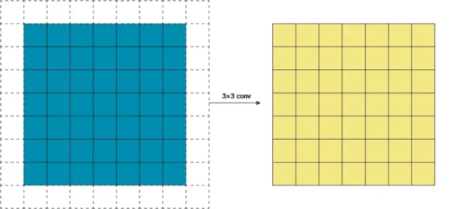
  • The convolution operation involves sliding the window of the convolution kernel at regular intervals, multiplying the elements of the convolution kernel at each position by the corresponding element of the input, and then summing (sometimes this computation is referred to as the product-accumulation operation), saving this result to the corresponding position of the output. The convolution operation is shown below:

    For a single image, the convolution kernel slides over each region of the image sequentially from the very beginning of the image, from left to right and from top to bottom, at a spacing of one pixel or specified number of pixels.

• The size of the convolution kernel ($f\times f$) can also be varied, for example$1\times 1、5\times 5$etc., at which point the Padding Size needs to be adjusted according to the size of the convolution kernel. Generally, the convolution kernel size is taken as an odd number (because we want the convolution kernel to have a center for processing the output). When the convolution kernel size is odd, the padding size can be determined according to the following formula:$PaddingSize=\frac{f-1}{2}$。

  Convolution kernels can be thought of as weights. Each convolution kernel can be regarded as a “feature extraction operator”, and the filtering result obtained by sliding an operator over the original map is called “Feature Map” (Feature Map), and these operators are called “Convolution Kernel” (Convolution Kernel). These operators are called “Convolution Kernel” (Convolution Kernel). Instead of designing these operators manually, we use random initialization to get many convolution kernels, and then optimize these convolution kernels by backpropagation to expect better recognition results.

• Padding/white-out (Padding)

  • Before proceeding with the convolutional layer, sometimes fixed data (e.g., 0, etc.) is filled in around the input data; the purpose of using padding is to resize the output so that the output dimension is the same as the input dimension;

    Without resizing, the output size will become very small after many layers of convolution. So, in order to minimize the loss of, edge information caused by the convolution operation, we need to perform padding (Padding).

• Stride/Length (Stride)

  • That is, the convolution kernel slides a few pixels at a time. In the previous section, we defaulted to sliding the convolution kernel one pixel at a time, but in fact, it is possible to slide two pixels at a time. The number of pixels slid at a time is called the “step size”. A convolution kernel with a step size of 2 is calculated as follows;

• If the output size is desired to be much smaller than the input size, measures can be taken to increase the step size. However, a step size of 2 cannot be used frequently, because if the output size becomes too small, a lot of information will inevitably be lost, even if the parameters of the convolution kernel are optimized well;

• If you use$f$denotes the convolution kernel size.$s$denotes the step size.$w$indicates the width of the image.$h$denotes the height of the image, then the output size can be expressed as:
  $$\begin{gathered} w_{out}=\frac{w+2\times PaddingSize-f}{s}+1 \\ {h}_{out}=\frac{h+2\times PaddingSize-f}{s}+1 \end{gathered}$$

• Filter

  • Convolution kernels (operators) are two-dimensional weight matrices; while filters (filters) are three-dimensional matrices stacked with multiple convolution kernels.

    In the case of only one channel (2D), a “convolution kernel” is equivalent to a “filter”, and the two concepts are interchangeable!

  • The convolution process above, did not consider the color image has RGB three-dimensional channel (Channel), if you consider the RGB channel, then each channel needs a convolution kernel, only when the calculation of the convolution kernelEach channel slides in the corresponding channelThe output is obtained by summing the computed results of the three channels. That is, each filterOne and only one output channel。

    As the individual convolutional kernels in the filter slide over the input data, they output different processing results, where some of the convolutional kernels may have a higher weight and the data in its corresponding channel is given more importance, with the filter focusing more on the feature differences in this channel.

• leaving one’s seat

  • Finally, the bias term and filter work together to produce the final output channel.

Multiple filters work in the same way: if there are multiple filters, we can then combine these final single-channel outputs into a total output whose number of channels is equal to the number of filters. This total output is then nonlinearly processed and fed as input to the next convolutional layer, and the process is repeated.

Therefore, there are a total of 4 hyperparameters in this section: the number of filters$K$Filter Size$F$footsteps$S$Zero fill size$P$。

2. Three modes of convolution

In fact, these three different modes are different restrictions on the range of movement of the convolutional kernel.

• **Full Mode:** Convolution is done from the time when the convolution kernel and the image are just intersected, and the white part is filled with zero.

• **Same Mode:** When the center of the convolution kernel (K) coincides with the edges of the image, it starts to do the convolution operation, and the white part is filled with 0. It can be seen that its range of motion is smaller than that of Full mode.

  Note: Same here also means that the size of the output feature map remains the same (relative to the input image) after convolution. Of course, same mode does not mean that the input and output sizes are exactly the same, but also has to do with the step size of the convolution kernel. same mode is also the most common mode, because this mode can keep the size of the feature map unchanged during the forward propagation process, and the tuner does not need to accurately calculate the change in its size (because the size does not change at all).

• **Valid Mode:** Convolution operations are performed when the convolution kernel is all inside the image, which is seen to move less than Same.

3. The nature of convolution

Primary sources for this section:List of commonly used convolution methods for CNN。

Going back to our roots, let’s go back to our math textbooks to look at convolution. In generalized functional analysis, a convolution, also known as a convolution or pleat product, is a process that passes two functions$x(t)$and$h(t)$generated mathematical operators. Its formula is as follows:
$$\begin{gathered} evenTo\; continueThe\; shapetype：x(t)h(t)(\tau )={\int }_{-\infty }^{+\infty }x(\tau )h(\tau -t)dt \\ From\; thescatteredThe\; shapetype：x(t)h(t)(\tau )=\sum _{\tau =-\infty }^{\infty }x(\tau )h(\tau -t) \end{gathered}$$
The convolution of two functions is to first flip (Reverse) one function and then do a translation (Shift), which is “volume“Meaning. And.”product“It is the multiplication of the corresponding elements of the two shifted functions to sum. So convolution is essentially a Reverse-Shift-Weighted Summation operation.

Convolution can better extract regional features, using different sizes of convolution operators can extract features at all scales of the image. Convolution has a wide range of applications in signal processing, image processing and other fields.

3.2.3 Pooling layer

Pooling, also known as aggregation in some places, is actually anDown-sampleprocess, which is used to reduce the size in the height and length directions, reduce the model size, and increase the computing speed, while improving the robustness of the extracted features. In simple terms, it is designed to extract the main features of a certain region and reduce the number of parameters to prevent model overfitting.

Pooling layers usually appear after convolutional layers, the two alternate with each other, and each convolutional layer corresponds to a pooling layer.

Commonly used pooling functions are: Average Pooling (Average Pooling / Mean Pooling), Maximum Pooling (Max Pooling), Minimum Pooling (Min Pooling) and Stochastic Pooling (Stochastic Pooling), etc., of which three types of pooling are shown below.

Each of the three pooling methods has its own advantages and disadvantages. Mean pooling averages all feature points, while maximum pooling maximizes the value of a feature point. Random pooling, on the other hand, is in between, by assigning probabilities to pixel points according to their numerical magnitude, and then subsampling them according to the probabilities, which, in the average sense, is approximate to mean sampling, and in the local sense, obeys the criterion of maximum sampling.

According to Boureau’s theory²It can be concluded that in the process of feature extraction, mean pooling can reduce the variance of the estimated value caused by the restricted size of the neighborhood, but retains more of the image background information; while maximum pooling can reduce the deviation of the estimated mean value error caused by the parameter error of the convolutional layer, and retains more of the texture information. Although random pooling can retain the information of mean pooling, but the random probability value is indeed added artificially, and the setting of random probability has a large impact on the results, which cannot be estimated.

The pooling operation also has a convolutional kernel-like thing moving around the feature map, which the book calls a pooling window³, so this pooling window also has a size, a step size when moving, and a fill operation before pooling. Therefore, the pooling operation also has a kernel size$f$step$s$padding$p$parameter, which has the same meaning as convolution.Max pooling is performed as follows (the pooling window is$2\times 2$, no padding, and a step size of$2$)：

Generally, the pooling window size will be set to the same value as the step size.

The pooling layer has three characteristics:

• There are no parameters to learn, which is different from the pooling layer. Pooling just takes the maximum or average value from the target region, so there is no need to have learned parameters.
• The number of channels does not change, i.e., it does not change the number of Feature Maps.
• It uses the principle of local correlation of images to subsample the image so that it is robust to small positional changes – pooling will still return the same result when the input data is slightly deviated.

3.2.4 Activation layer

That is, using an activation function that introduces nonlinearity into the model. For a specific introduction to the function, see the first post:Study Note: Deep Learning (1) – Basic Concepts and Activation Functions。

3.2.5 Rasterization

Rasterization: in order to be fully connected to the traditional multilayer perceptron MLP, each pixel of all the Feature Maps of the previous layer is expanded in turn and lined up in a column. This layer can be omitted in some cases.

Rasterization is the process of converting vertex data into tessellations and has the effect of transforming the graph into arasterThe role of the composed image is characterized by the fact that each element corresponds to one pixel in the frame buffer.

3.2.6 Full connectivity layer

I.e., picking up a traditional neural network, you can read the second article:Study Notes: Deep Learning (2) – BP Neural Networks。

3.2.7 Reverse propagation

Anyone who has tried to write their own neural network code from scratch knows that completing forward propagation isn’t even halfway through the entire algorithmic process. The real fun comes when you want to do backpropagation.

The principle of the BP algorithm for backpropagation can likewise be seen in the second article:Study Notes: Deep Learning (2) – BP Neural Networks。

The mathematical derivation of backpropagation for multilayer perceptrons is mainly represented by mathematical formulas, which are not complicated in fully connected neural networks, and are better understood even in pure mathematical formulas, while theBackpropagation of Convolutional Neural NetworksRelatively complex.

• Backpropagation of pooling layers

Backpropagation in the pooling layer is easier to understand, and we use maximum pooling as an example:

In the above figure, the number 6 after pooling corresponds to the red region before pooling, in fact, only the maximum number 6 in the red region has an effect on the result after pooling, with a weight of 1, while all other numbers have an effect of 0. Assuming that the error in the position of the number 6 after pooling is$\delta$The position error corresponding to the maximum value in the red region when back propagating back is equal to$\delta$, while the other 3 positions correspond to an error of zero.

Therefore, when maximally pooling forward propagation in a convolutional neural network, it is important to record not only the maximum value of the region but also theRecord the location of the region’s maximum valuethat facilitates back propagation of errors.

And average pooling is even simpler, since with average pooling, the weight of each value in the region contributing to the pooled result is the inverse of the region size, so the backpropagation comes back with an error at each location in the region ofpost-pooling errordivided bySize of the area。

• Backpropagation of convolutional layers

Although the convolution operation of a convolutional neural network is a convolution operation between a three-dimensional tensor picture and a four-dimensional tensor convolution kernel, the most central computation involves only a two-dimensional convolution, so we start with the two-dimensional convolution operation:

As shown above, when we find the error at the original figure A, we first analyze, which nodes in the next layer it affects in the forward propagation. Obviously, it only has an effect of weight B on node C and has no effect on any other node in the convolution result. Therefore the error of A should be equal to the error of point C multiplied by the weight B.

We now move the position of point A of the original figure, then point A influences point D of the convolution result with weight C and point E of the convolution result with weight B. Then its error is equal to the error of point D multiplied by C plus the error of point E multiplied by B. Then its error is equal to the error of point D multiplied by C plus the error of point E multiplied by B. You can try to use the same method to analyze the error of other nodes in the original graph, and you will find that the error of the original graph is equal to the delta error of the convolution result.Zero-filltreated withConvolutional kernel rotated 180 degreesPost-convolution.

The conclusions so far are still only based on 2D convolution, and we still need to generalize it to the convolution of tensors in our convolutional neural network. Recalling the convolution of a tensor again, each channel of the latter layer is obtained by convolving and then summing the individual channels of the previous layer. The first$Ⅰ$The channel 1 of the layer influences the first by convolution of the$Ⅰ+1$channels 1 and 2 of the layer, then solve for the first$Ⅰ$When the error of the layer channel 1, it is time to propagate the error of the 2D convolution according to the way of the error propagation of the obtained 2D convolution of the first$Ⅰ+1$The errors in layer channel 1 and channel 2 propagate to the first$Ⅰ$The errors in the layers are simplylook for a draw (chess)Ready to go.

Summarize the training process of convolutional neural networks:

1. Initialize the neural network, define the network structure, set the activation function, convolution kernel for convolutional layer$W$deviation$b$Perform stochastic priming for the weight matrix of the fully connected layer$W$and bias$b$Perform random initialization.
   Set the maximum number of iterations for each training$batch$The size of the learning rate$\eta$。

2. From the training data, a$batch$data from that$batch$A data is taken out of the data, including the input$x$and the corresponding correct labeling$y$。

3. switches the input$x$fed to the inputs of the neural network to obtain the output parameters of each layer of the neural network$z^l$and$a^l$。

4. Based on the output of the neural network and the labeled values$y$Compute the loss function of a neural network$Loss$。

5. Calculate the loss function$Loss$Errors to the output layer${\delta }^L$。

6. Use the recursive formula for the error between neighboring layers to find the error for each layer:

   • If it is a fully connected layer:${\delta }^l={\sigma }^{\prime }\cdot z^l=(W^{l+1}{)}^T\cdot {\delta }^{l+1}$；
   • If it is a convolutional layer:${\delta }^l={\sigma }^{\prime }\cdot z^l={\delta }^{l+1}\cdot ROT180(w^{l+1})$；
   • If it’s a pooling layer:${\delta }^l={\sigma }^{\prime }\cdot z^l=upsample({\delta }^{l+1})$。

7. The delta error of each layer is used to find the derivative of the loss function with respect to the parameters of that layer:

   • If it is a fully connected layer:$\frac{\partial C}{\partial W^l}={\delta }^l(a^{l-1}{)}^T,\frac{\partial C}{\partial b^l}={\delta }^l$；
   • If it is a convolutional layer:$\frac{\partial C}{\partial w^l}={\delta }^l\cdot \sigma (z^{l-1}),\frac{\partial C}{\partial b^l}={\sum }_x{\sum }_y{\delta }^l$。

8. Add the resulting derivative to this$batch$on the sum of the derivatives obtained from the data (initialized to 0), jump to step 3 until the$batch$The data are trained.

9. Using a$batch$The sum of the derivatives obtained from the data is used to update the parameters according to the gradient descent method:

   $W^l=W^l-\frac{\eta }{batch\_size}\sum \frac{\partial C}{\partial W^l}$，$b^l=b^l-\frac{\eta }{batch\_size}\sum \frac{\partial C}{\partial b^l}$。

10. Jump to step 2 until the specified number of iterations is reached.

3.2.8 Characteristics of CNNs

The special characteristics of convolutional neural networks compared to other traditional neural networks are mainly the followingpower sharingwithlocal connectionTwo aspects.

Addendum: Convolution is still a linear transformation(Source:What is convolution for deep learning?）：

Although the mechanism of convolutional layers has been explained above, we have not been able to explain why convolution can be scaled and why it works so well on image data. Suppose we have a 4×4 input and the goal is to convert it into a 2×2 output.

At this point, if we were using a feed-forward network, we would reconvert this 4×4 input into a vector of length 16, and then feed these 16 values into a densely connected layer with 4 outputs. Here is the weight matrix W for this layer:

While the convolutional kernel operation of convolution may seem strange, it is still a linear transformation with an equivalent transformation matrix. If we use a convolution kernel K of size 3 on the reconstructed 4×4 input, then this equivalent matrix becomes:

It can be noticed that the whole convolution is still a linear transformation, but at the same time, it is a very different transformation. Compared to the 64 parameters of the feedforward network, the 9 parameters obtained by convolution can be reused many times. Since the weight matrix contains a large number of 0 weights, we will only see a selected number of inputs (inputs to the convolution kernel) at each output node.

And more efficiently, the predefined parameters of the convolution can be considered as a priori for the weight matrix. When we use a pre-trained model for image classification, we can use the pre-trained network parameters as the current network parameters and train our own feature extractor based on them. This will save a lot of time.

In this sense, the advantage of convolution over feedforward networks can be explained, although it is the same linear transformation. Unlike random initialization, the use of pre-trained parameters allows us to optimize only the parameters of the final fully connected layer, which means better performance. And cutting the number of parameters considerably means higher efficiency.

1. Localized connectivity/connection pruning/sparse connectivity (Sparse Connectivity)

Hubel and Wiesel, 1962.⁴The concept of receptive fields was developed by studying the visual hierarchy in biological neurology, where visual neurons in the cerebral cortex perceive information based on localized regional stimuli. The idea of local area connections is inspired by the structure of visual neurons.

In the traditional neural network structure, the connection between neurons is fully connected, i.e., the neurons in the n-1 layer are connected to all the neurons in the n layer, so any unit in the output is affected by all the units in the input, which will invariably reduce the recognition effect of the image; however, in the convolutional neural network, any unit in the output image is only related to a part of the input image, and the number of connections is reduced exponentially. relationship, the number of connections is reduced exponentially, and the corresponding parameters are also reduced.

2. Authority sharing/parameters sharing (Parameters Sharing)

Primary sources for this section:An overview of convolutional neural networks。

1998, LeCun⁵released the LeNet-5 network architecture, the term weight sharing was first coined by the LeNet-5 model. Although most people now believe that the 2012 AlexNet network⁶is the beginning of deep learning, but the beginnings of CNNs can be traced back to the LeNet-5 model.Several features of the LeNet-5 model were widely used in the early 2010’s in the study of convolutional neural networks, one of which was weight sharing.

In a convolutional neural network, the convolutional kernel (or called a filter) in the convolutional layer is similar to a sliding window that slides back and forth in the entire input image in a specific step size, and after the convolution operation, thus obtaining the feature map of the input image, which is the local features extracted by the convolutional layer, and theThis convolution kernel is shared parameter. The convolution kernel containing the weights is updated throughout the training of the network until training is complete.

• What is weight sharing?
  • Actually weight sharing is when the whole image is using parameters within the same convolutional kernel. For example, a 33A convolution kernel of 1. The parameters of 9 of this convolution kernel are shared by the entire image without changing the weight coefficients within the convolution kernel due to different positions within the image. To put it more plainly, a convolutional kernel is used to convolve an entire image without changing the weights within the kernel.
  • Of course, there won’t be just one convolutional kernel per convolutional layer in a CNN, and that’s just for ease of explanation.
• Advantages of weight sharing?
  • The weight-sharing convolutional operation ensures that each pixel has a weight coefficient, except that these coefficients are shared by the entire image, thus greatly reducing the number of parameters in the convolutional kernel and decreasing the complexity of the network;
  • Traditional neural networks and machine learning methods require complex pre-processing of the image to extract features, and the obtained features are then fed into the neural network. Instead, adding convolutional operations allows features to be extracted automatically by utilizing local correlations on the image space;
  • Similarly, due to the parameter sharing of the filter, we can still recognize features even if the image undergoes some panning operation, which is called “panning invariance”. As a result, the model is much more robust.
• Why do convolutional layers have multiple convolutional kernels?
  • Because weight sharing means thatEach convolutional kernel can extract only one type of feature, in order to increase the expressive power of the CNN, multiple convolutional kernels need to be set up. However, the number of convolution kernels/filters in each convolutional layer is a hyperparameter.

3. Receptive Field – Visualization of CNNs

Regardless of the CNN architecture, their basic design is to constantly compress the height and width of the image while increasing the number of channels, or depth. The localization affects the input and output observation regions of the neighboring layers, while the sensory field determines theObservation region for the original input of the entire network。

**Receptive Field** is defined as the size of the region in which the pixels on the feature map output by each layer of a convolutional neural network are mapped on the input image. I.e., the input area that the neurons in the neural network “see”. In a convolutional neural network, the computation of an element of the feature map is affected by a certain area of the input image, which is the receptive field of that element. A more general explanation is that a point on the feature map corresponds to a region on the input map, as shown in the figure.

After adjusting the stride to 2, the output obtained from the convolution shrinks considerably. At this point, if we do a nonlinear activation on top of this output and then add another convolutional layer on top of it, something interesting happens. The 3×3 convolution kernel has a much larger sense of wildness on this step-wise convolution output compared to the output obtained from normal convolution. This is shown in the figure below:

This is because its original input region is then larger than the input region of a normal convolution, and this expansion of the sensory field allows the convolutional layers to combine low-level features (lines, edges) into higher-level features (curves, textures), as we saw in the mixed3a layer. And as we add more Stride layers, the network displays more high-level features, such as mixed4a, mixed5a.

By detecting low-level features and using them to detect higher-level features that move forward in the visual hierarchy, it is eventually possible to detect entire visual concepts such as faces, birds, trees, etc. This is one reason why convolution is so powerful and efficient on image data.

The specific calculation of the receptive field can be referred to: [thoroughly understand the meaning and calculation of the receptive field](https ~:text=Receptive field (Receptive,Field), refers to the neuron in the neural network neurons “see” the input region, in the convolutional neural network, the feature map on a certain element of the calculation is affected by a region of the input image, this region is the element of the receptive field. In a convolutional neural network, the computation of an element of the feature map is affected by a region of the input image, which is the receptive field of that element). In a convolutional neural network, the computation of an element of the feature map is affected by a region of the input image that is the receptive field of that element.

3.2.9 CNN generalization ability improvement techniques

• Increase neural network depth;

• Modification of the activation function, the more used is the ReLU activation function;

• Adjusting the weight initialization technique, in general, a uniformly distributed initialization works better;

• Adjusts the batch size (dataset size);

• Extending the dataset (data augmentation), you can extend the dataset by panning, rotating the image, etc. to make the learning effect better;

• Take regularization;

• Dropout method is taken to avoid overfitting.

3.3 Overview of types of CNNs

This review categorizes recent CNN architectural innovations into seven different categories based on space utilization, depth, multipath, width, feature map utilization, channel boosting, and attention [^12].

CNNs first gained attention through LeCun’s 1989 work with lattice-like topological data (images and time-series data.) Considered as one of the best techniques for understanding the content of images and showing the best current performance on tasks related to image recognition, segmentation, detection, and retrieval, the success of CNNs has attracted attention outside of academia. In industry, companies such as Google, Microsoft, AT&T, NEC, and Facebook have established research teams to explore new architectures for CNNs. Currently, most of the frontrunners in the image processing race use deep CNN-based models.

Since 2012, different innovations on CNN architecture have been proposed. These innovations can be categorized as parameter optimization, regularization, restructuring, etc. However, it has been observed that the performance improvement of CNN networks should be mainly attributed to the reconfiguration of the processing units and the design of new modules.

CNN-based applications have become increasingly popular since AlexNet demonstrated exceptional performance on the ImageNet dataset. Similarly, Zeiler and Fergus introduced the concept of feature hierarchical visualization, which changed the trend of extracting features in simple low spatial resolution with deep architectures such as VGG. Today, most new architectures are built based on the simple principles and homogenized topologies introduced by VGG.

On the other hand, Google team introduced a very famous concept about splitting, transforming and merging called Inception block. The initial block used for the first time the concept of intra-layer branching, allowing the extraction of features at different spatial scales.In 2015, the concept of residual connectivity introduced by Resnet in order to train deep CNNs became famous and, it is used by most of the later networks like Inception-ResNet, WideResNet, ResNext, etc. Similarly, some architectures like WideResnet, Pyramidal Nets, Xception introduced the concept of multilayer transformations by means of extra bases and increased width. As a result, the focus of research has shifted from parameter optimization and connection re-tuning to network architecture design (layer structure). This has given rise to many new architectural concepts like channel boosting, space and channel utilization, attention-based information processing, etc.

There have been many different improvements to the CNN architecture since 1989 to the present day.All innovations in CNNs have been realized by combining depth and space. Based on the type of architectural modifications, CNNs can be broadly categorized into 7 classes:CNN based on space utilization, depth, multipath, width, channel boosting, feature map utilization and attention. The classification of the deep CNN architecture is shown in Fig.

3.3.1 CNN based on space utilization

CNNs have a large number of parameters such as the number of processing units (neurons), number of layers, filter size, step size, learning rate and activation function. Since CNNs consider the neighborhood (locality) of the input pixels, different filter sizes can be used to explore different levels of correlation. Therefore, in the early 2000s, researchers utilized spatial transformations to improve performance, in addition to evaluating the effect of different sized filters on the network’s learning rate. Different filter sizes encapsulate different levels of granularity; typically, smaller filters extract fine-grained information while larger filters extract coarse-grained information. In this way, by adjusting the filter size, the CNN can perform well in both coarse- and fine-grained details.

CNNs based on spatial exploitation (Spatial Exploitation based) are LeNet, Alenet, ZefNet, VGG, GoogleNet and so on.

1. LeNet-5（20c90s）

LeNet was one of the first convolutional neural networks to advance the field of deep learning. This project, developed by Yann LeCun⁷The pioneering work accomplished has been named LeNet-5 after many successful iterations since 1988. (The model is essentially the same as described above.)

convolutional layerThe basic unit in the block is a convolutional layer backed by an average pooling layer. Each convolutional layer uses a 5 × 5 window on the output of theSigmoidactivation function, which is used to recognize spatial patterns in the image, such as lines and object localization (the first convolutional layer outputs a number of channels of 6, while the second convolutional layer outputs an increased number of channels of 16); and an average pooling layer is used to reduce the sensitivity of the convolutional layer to position, sample the output of the convolutional layer, and compress the size of the image dimensions. The convolutional layer consists of two such basic units stacked repeatedly.

full connectivity layerThe block contains 3 fully connected layers. The vectors in them are all expanded into one-dimensional vectors, and the one-dimensional vectors are dot-producted with the weight vectors, with a bias added, and output after passing through the activation function to get the new neuron output. Their number of neurons are 120, 84 and 10 respectively, where 10 is the number of categories of the output and also the output layer.

2. AlexNet（2012）

2012, Alex Krizhevsky et al.⁶released AlexNet, which is a boosted depth and breadth version of LeNet, and won the ImageNet Large Scale Visual Recognition Challenge (ILSVRC) in 2012 by a huge margin. This was a major breakthrough based on previous methods, and the current widespread use of CNNs is all thanks to AlexNet.

AlexNet demonstrated for the first time that learned features can outperform hand-designed features with the following four features:

• An 8-layer transform with 5 convolutional and 2 fully-connected hidden layers, and 1 fully-connected output layer;
• Changing the sigmoid activation function to a simpler ReLU activation function reduces the computational complexity of the model and increases the training speed of the model by several times;
• Max pooling to avoid the blurring effect of average pooling. Overlap pooling is also used to improve the richness of features;
• Controlling the model complexity of the fully connected layer with Dropout: Some neurons in the intermediate layer are randomly set to 0 during the training process by the Dropout technique, which makes the model more robust and also reduces the overfitting of the fully connected layer;
• Data Augmentation such as image panning, mirroring, flipping, cropping, changing grayscale and color variations are introduced to further expand the dataset to mitigate overfitting.
  

3. GoogLeNet（2014）

The 2014 ILSVRC winners are Google’s Szegedy et al.⁸Human Convolutional Networks. Its main contribution was the development of an initial module (Inception) that significantly reduces the number of parameters in the network (4M compared to 60M for AlexNet).

LeNet, AlexNet, and VGG all fully extract spatial features first with a block consisting of a convolutional layer, and then output classification results with a block consisting of a fully connected layer. Unlike their three models, the GoogLeNet model consists of the following Inception base block, which is equivalent to a sub-network with four lines, and the structure combines the commonly used convolution in CNNs ($1\times 1,3\times 3,5\times 5$), pooling operations (3×3) are stacked on top of each other to increase the width of the network on the one hand and its adaptability to scale on the other. It extracts information in parallel through convolutional and maximum pooling layers with different window shapes and uses the$1\times 1$The convolutional layer reduces the number of channels thereby reducing the model complexity. It has 12 times fewer parameters than AlexNet and GoogleNet is more accurate.

4. VGGNet（2014）

The 2014 ILSVRC runner-up was a network called VGGNet by Simonyan et al.⁹Development. Its main contribution is to demonstrate that network depth (number of layers) is a key factor in performance. It uses small convolutional kernels and replaces convolutional kernel size with convolutional depth.

The VGG model replaces a convolutional layer with a larger convolutional kernel with multiple convolutional layers with small convolutional kernels, e.g., with a convolutional layer of size both$3\times 3$The 3-layer convolutional layer of the convolutional kernel replaces a layer with a$7\times 7$convolutional layer of the convolutional kernel, this substitution reduces the number of parameters and also enables the decision function to be more discriminative. Picking up on a step size of$2$The shape of the window is$2\times 2$of the maximum pooling layer such that the convolutional layer keeps the height and width of the input constant, while the pooling layer halves it.

• 2$3\times 3$Equivalent to 1$5\times 5$ ；
• 3$3\times 3$Equivalent to 1$7\times 7$；
• $1\times 1$of the convolutional layer can be considered as a nonlinear transformation.

Experimental results show that the performance of the model can be effectively improved when the number of weighting layers reaches 16-19 layers. The most common ones are VGG16 and VGG19 models. Among them, the VGG16 network structure is as follows:

The VGG model obviously improves the performance of the model by increasing the number of layers and increasing the depth of the model, but there also exists the phenomenon of gradient explosion and gradient disappearance at the same time can not be solved; in addition, the model also suffers from the degradation problem, i.e., the depth of the model reaches 20 layers, in the increase of the depth of the model’s ability instead of decreasing.

3.3.2 Depth-based CNNs

The deep CNN architecture is based on the assumption that with increasing depth, the network can better approximate the objective function with a large number of nonlinear mappings and improved feature representations. Network depth plays an important role in the success of supervised learning. Theoretical studies have shown that deep networks are able to represent specific 20 function types exponentially more efficiently than shallow networks.In 2001, Csáji expressed the Generalized Approximation Theorem stating that a single hidden layer is sufficient to approximate any function, but that this requires exponentially more neurons and thus usually leads to computational infeasibility. In this regard, Bengio and elalleau argued that deeper networks have the potential to maintain the expressive power of the network at less cost. in 2013, Bengio et al. showed empirically that deep networks are computationally and statistically more efficient for complex tasks. Inception and VGG, the top performers in the 2014-ILSVR competition, further illustrate that depth is an important dimension that regulates the learning ability of networks.

Once a feature has been extracted, its extraction position becomes less important as long as its approximate position relative to other positions is preserved. Pooling or downsampling (e.g., convolution) is an interesting local operation. It summarizes similar information in the vicinity of the receptive field and outputs the dominant response within that local region. As an output of the convolution operation, the feature pattern may appear at different locations in the image.

Depth based CNNs are Highway Networks, ResNet, Inception V3/V4, Inception-ResNet, ResNext, and so on.

ResNets（2015）

Ho, K. M., et al.¹⁰human-developed residual networks was the 2015 ILSVRC winner.ResNets is the most advanced convolutional neural network model to date and is the default choice for everyone using convolutional neural networks in practice (as of May 2016).ResNets uses Residual Networks (ResNet) to solve the gradient vanishing Problem.

The main feature of ResNet is cross-layer connectivity, where inputs are passed across layers and added to the result of the convolution by introducing shortcut connections. There is only one pooling layer in ResNet, which is connected behind the last convolutional layer.ResNet allows the underlying network to be fully trained and the accuracy improves significantly with depth. ResNet with a depth of 152 layers was used in the image classification competition of LSVRC-15 and it got the 1st place. In this literature, an attempt was also made to set the depth of ResNet to 1000 and validate the model on the CIFAR-10 image processing dataset.

ResNe solves the degeneracy problem of VGGNet in the form of constant mapping:

The idea of residuals is to remove the same body parts so as to highlight the small changes, and the altered output changes are more effective in adjusting the weights, so they work better.

If the input is set to X, and a given parametric network layer is set to H, then the output of this layer with X as input will be H(X). General CNN networks such as Alexnet/VGG will learn the expression of the parametric function H directly through training, thus learning X -> H(X) directly. Residual learning, on the other hand, is dedicated to learning the covariance between inputs and outputs using multiple participatory network layers i.e., F(X) = H(X) – X, i.e., learning X -> F(X) + X. The X part of the network is the direct identity mapping while F(X) = H(X) – X is the residuals between inputs and outputs to be learned by the participatory network layers.

The deeper the layers of the network the richer the feature representation of the input image can be extracted. However, for previous non-residual networks, simply increasing the depth can lead to the problem of gradient dispersion or gradient explosion, whereas ResNet models have successfully solved the problem of network depth, and ResNet models can be made very deep, with some currently available even exceeding 1000 layers. Research and experiments have shown that deepened residual networks can be optimized more easily than deep networks produced by simply stacking layers, and the effectiveness of the model is significantly improved because of the increased depth. The network structure of one ResNet is shown below.

3.3.3 Multi-path based CNNs

Deep networks are challenging to train, which has been the subject of much recent deep network research. Deep CNNs provide efficient computation and statistics for complex tasks. However, deeper networks may suffer from performance degradation or gradient vanishing/exploding problems, which are usually caused by increasing depth rather than overfitting. The problem of vanishing gradients not only leads to higher testing errors, but also to higher training errors. To train deeper networks, the concept of multipath or cross-layer connections has been proposed. Multipath or shortcut connections can systematically connect one layer to another by skipping some intermediate layers in order to make a specific flow of information across the layers. Cross-layer connections divide the network into pieces. These paths also try to solve the gradient vanishing problem by making the gradient accessible to lower layers. For this purpose, different types of shortcut connections such as zero-padding, projection-based, dropout and 1×1 connections are used.

Multi-Path based (MPB) CNNs are Highway, ResNet, DenseNet, and so on.

3.3.4 Breadth-based multi-connected CNNs

From 2012 to 2015, the focus of network architecture is on the power of depth and the importance of multi-channel regulatory connectivity in network regularization. However, the width of the network is as important as the depth. By using multiple processing units in parallel within a layer, multilayer perceptrons gain the advantage of mapping complex functions on the perceptron. This suggests that width is as important a parameter in defining the learning principle as depth.Lu et al. and Hanin & Sellke have recently shown that neural networks with linear rectifier activation functions need to be wide enough to maintain generalized approximation properties with increasing depth. Moreover, continuous function classes on tight sets cannot be well approximated by networks of arbitrary depth if the maximum width of the network is not larger than the input dimension. Therefore, multilayer stacking (adding layers) may not increase the characterization ability of a neural network. An important issue related to deep architectures is that some layers or processing units may not be able to learn useful features. To address this issue, the focus of research has shifted from deep and narrower architectures to shallower and wider architectures.

Width based Multi-Connection (WideResNet, Pyramidal Net, Xception, Inception Family, etc.) CNNs.

3.3.5 CNN developed based on (channel) feature maps

CNNs are known for their hierarchical learning and automatic feature extraction capabilities in MV tasks. Feature selection plays an important role in determining the performance of classification, segmentation and detection modules. The performance of classification module in traditional feature extraction techniques is limited by the singularity of features. In contrast to traditional techniques, CNNs use multi-stage feature extraction where different types of features (called feature maps in CNNs) are extracted based on the assigned inputs. However, some feature maps have little or almost no target discrimination. Huge feature sets have noise effects that can lead to network overfitting. This suggests that, in addition to network engineering, the selection of class-specific feature maps is critical to improving the generalization performance of the network. In this section, feature maps and channels will be used interchangeably, as many researchers have used the term channel instead of feature map.

The CNNs developed based on (channel) Feature Map Exploitation based are Squeeze and Excitation, Competitive Squeeze and Excitation, etc.

3.3.6 CNN based on (input) channel utilization

Image characterization plays an important role in determining the performance of image processing algorithms. A good representation of an image defines the salient features of an image from a compact code. In different studies, different types of conventional filters are used to extract different levels of information from a single type of image. These different representations are used as inputs to the model to improve the performance.CNN is a good feature learner which automatically extracts discriminative features based on the problem. However, the learning of CNN depends on the input representations. If the input lacks diversity and category definition information, the performance of CNN as a discriminator suffers. For this reason, the concept of auxiliary learners is introduced into CNNs to enhance the input representation of the network.

CNNs based on (input) Channel Exploitation based are Channel Boosted CNN using TL and so on.

3.3.7 Attention-based CNNs

Different levels of abstraction play an important role in defining the discriminative ability of a neural network. In addition to this, the selection of contextually relevant features is also important for image localization and recognition. In the human visual system, this phenomenon is called attention. Humans observe the scene and pay attention to the contextually relevant parts in one hurried glance after another. In this process, humans not only pay attention to the selected area but also reason out different interpretations about the objects at that location. Thus, it helps humans to grasp visual structures in a better way. Similar explanatory abilities are added to neural networks like RNN and LSTM. The above networks utilize the attention module to generate sequential data and weight new samples based on their occurrence in previous iterations. Different researchers have added the concept of attention to CNNs to improve the representation and overcome the computational limitations of the data. The concept of attention helps to make CNNs smarter so that they can recognize objects even in cluttered backgrounds and complex scenes.

Attention based CNN has: Residual Attention Neural Network, Convolutional Block Attention, Concurrent Squeeze and Excitation.

3.3.8 Addendum: PyTorch-Networks

For various CNN models, there have been PyTorch implementations of all of them: https //github.com/BIGBALLON/CIFAR-ZOO.

This series of convolutional neural network implementations contains 9 major topics, with: typical networks, lightweight networks, target detection networks, semantic segmentation networks, instance segmentation networks, face detection and recognition networks, human gesture recognition networks, attention mechanism networks, and portrait segmentation networks.

1. Classical network

• Typical CNN inclusions: AlexNet, VGG, ResNet, InceptionV1, InceptionV2, InceptionV3, InceptionV4, Inception-ResNet.

2. Light weight network (LWN)

• Lightweight network included:GhostNet、MobileNets、MobileNetV2、MobileNetV3、ShuffleNet、ShuffleNet V2、SqueezeNet Xception MixNet GhostNet。
  • MobileNet, proposed by Google in 2017, is a lightweight CNN neural network that focuses on being used on mobile and embedded devices, and has rapidly spawned three versions, v1 v2 v3; compared to traditional CNN networks, it greatly reduces the model parameters and the amount of computation with a small reduction in accuracy.
  • The main idea is no longer to improve the depth and width of the model, but to change the way of convolution, replace the standard convolution layer with depth separable convolution, that is, the convolution is divided into depth convolution and point-by-point convolution of the two steps, under the premise of guaranteeing the accuracy of the model, greatly reducing the model’s arithmetic. The comparison of the convolution process before and after the improvement is as follows:
    

3. Target detection network (Object Detection)

• The target detection network consists of SSDs,YOLO、YOLOv2、YOLOv3、FCOS、FPN、RetinaNet Objects as Points、FSAF、CenterNet FoveaBox。
  • Take YOLO series for example, YOLO (You Only Look Once) is a deep neural network based object recognition and localization algorithm, its biggest feature is that it runs very fast and can be used in real-time systems. Currently, YOLOv3 is more widely used.
    

4. Semantic Segmentation Network (SSN)

• The semantic segmentation network includes:FCN、Fast-SCNN、LEDNet、LRNNet、FisheyeMODNet。
  • As an example, FCN was born in 2014 as a pioneer of semantic segmentation models, and its main contribution is to popularize the use of end-to-end convolutional neural networks in semantic segmentation problems using inverse convolution for up-sampling.The FCN model is very simple, and all of the inside consists of convolutions, which is why it is called a fully-convolutional network, and also because of the special form of the fully-convolutional convolutions, it can accept inputs of arbitrary sizes.
    

5. Instance Segmentation (ISSN)

• Example segmentation networks include PolarMask.

6. Face detection and recognition network (commit VarGFaceNet)

• Face detection and recognition networks include FaceBoxes, LFFD, VarGFaceNet.

7. Human Pose Estimation (HPE) network

• Human posture recognition networks include Stacked Hourglass, Networks Simple Baselines, and LPN.

8. Network of Attention Mechanisms (Attention)

• Attention mechanism networks include SE Net, scSE, NL Net, GCNet, CBAM.

9. Portrait Segmentation Network (PSN)

• Portrait segmentation networks include SINet.

3.4 Limitations of CNNs

While these features that CNNs possess have led to their use in a wide variety of applications, their advantages do not mean that the networks that currently exist are without flaws.

How to effectively train deep network models with very deep layers is still a problem to be investigated. Although image classification tasks can benefit from deeper layers of convolutional networks, some methods still do not deal well with problems such as occlusion or motion blur.

Note: All images and animations used in the text belong to their respective authors.

---

1. ZHOU Feiyan, JIN Linpeng, DONG Jun. A review of convolutional neural network research[J]. Journal of Computing, 2017, 40(6): 1229-1251.↩︎

2. Boureau Y L, Bach F, LeCun Y, et al. Learning mid-level features for recognition[J]. 2010. ↩︎

3. An Introduction to Deep Learning Based on Python Theory and Implementation↩︎

4. Hubel D H, Wiesel T N. Receptive fields, binocular interaction and functional architecture in the cat’s visual cortex[J]. The Journal of physiology, 1962, 160(1): 106-154. ↩︎

5. LeCun Y, Bottou L, Bengio Y, et al. Gradient-based learning applied to document recognition[J]. Proceedings of the IEEE, 1998, 86(11): 2278-2324. ↩︎

6. Krizhevsky A, Sutskever I, Hinton G E. Imagenet classification with deep convolutional neural networks[C]//Advances in neural information processing systems. 2012: 1097-1105. https://www.aminer.cn/archive/imagenet-classification-with-deep-convolutional-neural-networks/53e9a281b7602d9702b88a98 ↩︎ ↩︎

7. https://arxiv.org/abs/1901.06032 ↩︎

8. Szegedy C, Liu W, Jia Y, et al. Going deeper with convolutions[C]//Proceedings of the IEEE conference on computer vision and pattern recognition. 2015: 1-9. ↩︎

9. Simonyan K, Zisserman A. Very deep convolutional networks for large-scale image recognition[J]. arXiv preprint arXiv:1409.1556, 2014. ↩︎

10. He K, Zhang X, Ren S, et al. Deep residual learning for image recognition[C]//Proceedings of the IEEE conference on computer vision and pattern recognition. 2016: 770-778. ↩︎