Neural Networks and Model Training Process in Detail

0. Preface

Artificial Neural Networks (Artificial Neural Network, ANN) is a supervised learning algorithm inspired by the way the human brain works. Similar to the way neurons are connected and activated in the human brain, a neural network receives inputs that are passed through the network by means of certain functions, leading to the activation of certain subsequent neurons that produce outputs. The more complex the function, the greater the network’s ability to fit the input data, and therefore the greater the accuracy of the prediction.
There are many differentANN architecture, according to the Generalized Approximation Theorem, we can always find a large enough neural network architecture containing the correct set of weights that can accurately predict the output result for any given input. This means that for a given dataset/task, we can create an architecture and keep adjusting its weights until theANN The process of predicting the correct result and adjusting the weights of the network is called training the neural network.
An important task in computer vision is the recognition of object classes in an image, i.e., image classification, theImageNet It is a prestigious competition in the field of image classification, and the classification accuracies in the past years are as follows:

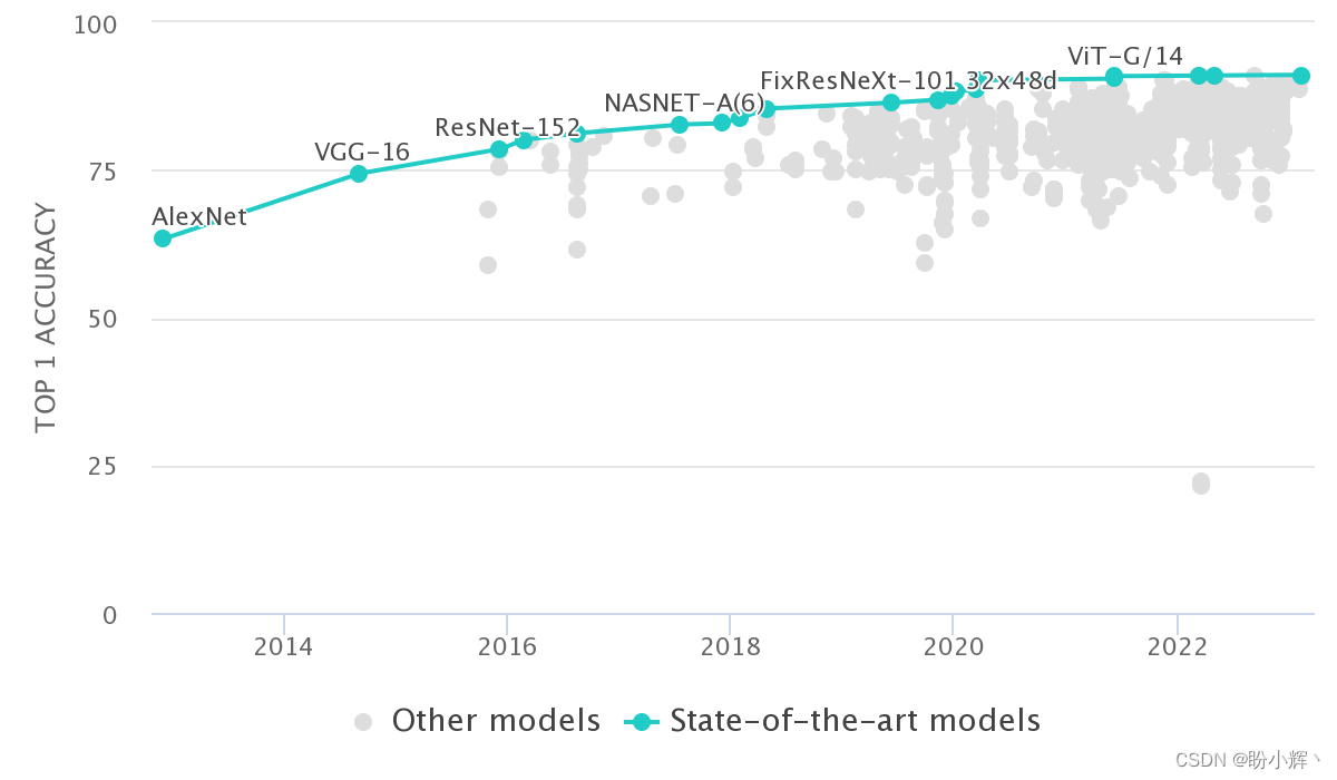
As can be seen from the above figure, by utilizing neural networks, the model error rate is significantly reduced, and as the neural networks gradually become deeper and more complex over time, the classification error rate continues to decrease and outperforms humans.
In this section, we will create a simple neural network architecture using a simple dataset to understand theANN of each component (forward propagation, backpropagation, learning rate, etc.) for model weight adjustment in order to grasp how neural networks learn to predict outputs based on given inputs. We will first introduce the math behind neural networks, then build a neural network from scratch and describe each component used to train the neural network.

1. Traditional machine learning and artificial intelligence

In traditional applications, systems are made intelligent by using complex algorithms written by programmers. For example, suppose we wish to recognize whether a photo contains a dog. In traditional machine learning (Machine Learning, ML) in which machine learning researchers are required to first determine the features that need to be extracted from an image, then extract those features and pass them as input to a complex algorithm that parses the given features to determine whether the image contains a dog:

However, if features are to be extracted manually for multiple categories of image classification, their number can be exponential, and therefore, traditional methods work well in restricted environments (e.g., recognizing photo IDs) and not so well in unrestricted environments, where there are large variations from one image to the next.
We can extend the same idea to other domains, such as text or structured data. In the past, if one wished to solve real-world tasks programmatically, one had to know everything about the input data and write as many rules as possible to cover all scenarios, with no guarantee that all new scenarios would follow the existing rules.
Neural networks, on the other hand, have the process of feature extraction built in and use these features for classification/regression, requiring little to no manual feature engineering, only labeling of the data (e.g., which images are dogs and which are not) and the neural network architecture, and no need to manually come up with rules to classify the images, which alleviates much of the burden imposed on programmers by traditional machine learning techniques.
Training a neural network requires the provision of a large amount of sample data. For example, in the previous example, we need to provide the model with a large number of dog and non-dog pictures so that it can learn the features. The process of neural networks for classification tasks is as follows, and their training and testing is end-to-end (end-to-end):

2. Basics of artificial neural networks

2.1 Artificial Neural Network Composition

ANN is the tensor (the weights, theweights ) and a collection of mathematical operations in an arrangement that approximates a loose arrangement of neurons in the human brain. It can be thought of as a mathematical function that takes one or more tensors as input and predicts the corresponding output (one or more tensors). The way in which the inputs are connected to the outputs operates is known as the architecture of the neural network, and we can build different architectures for different tasks, i.e., based on whether the problem consists of structured or unstructured (image, text, speech) data, which are lists of input and output tensors.ANN It consists of the following parts:

• Input layer: using independent variables as inputs
• Hidden (intermediate) layer: connects the input and output layers and performs transformations on top of the input data; in addition, the hidden layer utilizes the node units (circles in the figure below) to modify its input values to higher/lower dimensional values; a complex representation function can be implemented by modifying the activation function of the intermediate nodes
• Output layer: values generated by input variables

In summary, the typical structure of a neural network is as follows:

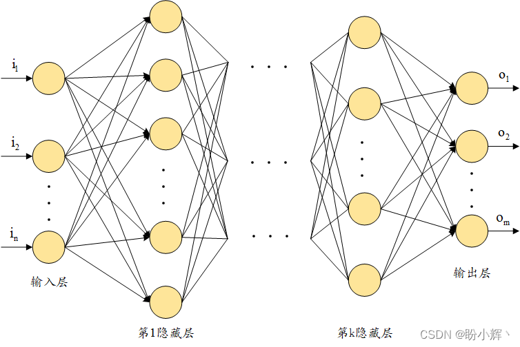
The number of nodes in the output layer (circles in the figure above) depends on the actual task and whether we are trying to predict continuous or categorical variables. If the output is a continuous variable, the output has one node. If the output is a variable withm categorization of the possible categories, there will be in the output layerm Nodes. Next, we delve into the workings of the node/neuron, where the neuron transforms its inputs as follows:

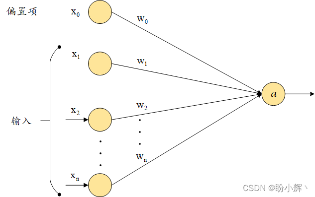
Among them.$x_1$，$x_2$，…，$x_n$ is the input variable.$w_0$ is the bias term (similar to bias in linear/logistic regression);$w_1$，$w_2$，…，$w_n$ is the weight assigned to each input variable and the output value$a$ The calculations are as follows:

$$a=f(w_0+\sum _{w_i}^N{w}_i{x}_i)$$

As can be seen.$a$ is the sum of the products of the weights and the input pairs, after which an additional function is used$f(w_0+{\sum }_{w_i}^N{w}_i{x}_i)$function$f$ is a nonlinear activation function applied on top of the sum of products for introducing nonlinearity in the sum of inputs and their corresponding weight values, which can be achieved by using multiple hidden layers for stronger nonlinear capabilities.
Overall, a neural network is a collection of nodes, where each node has a tunable floating-point value (weight) and the nodes are interconnected to return an output determined by the network architecture. The network consists of three main parts: an input layer, a hidden layer, and an output layer. We can use multiple layers (n) Hidden Layers, Deep Learning usually denotes a neural network with multiple hidden layers. Typically, more hidden layers are necessary when the neural network needs to learn tasks with complex contexts or contexts that are not obvious (e.g., image recognition).

2.2 Training of Neural Networks

Training a neural network is actually adjusting the weights in the neural network by repeating two key steps: forward propagation and back propagation.

1. In the forward propagation (feedforward propagation) in which we apply a set of weights to the input data, pass it to the hidden layer, use nonlinear activation on the computed output of the hidden layer, and after passing through a number of hidden layers, multiply the output of the last hidden layer with another set of weights to get the result of the output layer. For the first forward propagation, the values of the weights will be randomly initialized
2. In the case of backpropagation (backpropagation) in an attempt to reduce the error by measuring the output and then adjusting the weights accordingly. The neural network repeats forward and backward propagation to predict the output until it obtains weights that make the error smaller

3. Forward dissemination

To further understand how forward propagation works, we will construct a neural network through a simple example where the inputs to the neural network are(1,1)and the corresponding (expected) output is0, we find the optimal weights for the neural network based on this input-output pair. In an actual neural network, tens of thousands of data sample points are used for training.
The strategy we used is as follows: the neural network has a hidden layer, an input layer and an output layer, where the hidden layer contains three nodes as shown below:

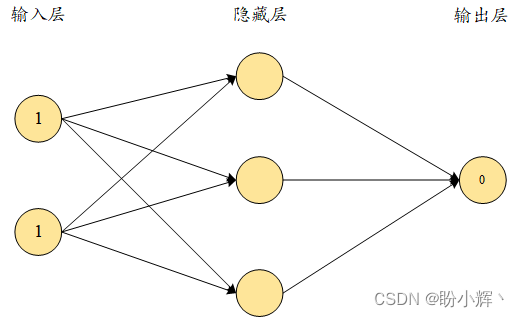
In the figure above, each arrow contains an adjustable floating point value (weight). We need to find the9 A floating-point number, when the input is(1,1) When the output is as close as possible to0This is the purpose of training the neural network (to get the output as close as possible to the target value). For simplicity, we did not introduce a bias term in the hidden layer cells. Next, we will introduce the following for the above network:

• Calculate hidden layer values
• Performs nonlinear activation
• Calculate output layer values
• Calculation of the value of the loss

3.1 Calculating hidden layer values

First, random weights are assigned to all connections; typically, neural networks are initialized with random weights before training begins. For simplicity, in this section, bias values are not included for forward and backward propagation.
The initial weights can be randomly initialized to0-1 between, but the final weights after the neural network training process do not need to be in a specific interval. A visual representation of the weights and values in the network is given on the left side of the figure below, and the randomly initialized weights in the network are given on the right side:

Next, the inputs are multiplied with the weights to calculate the values in the hidden layer. Before applying the activation function, the unit values in the hidden layer are as follows:
$$\begin{gathered} h_{11}=x_1\ast w_{11}+x_2\ast w_{21}=1\ast 0.8+1\ast 0.2=1 \\ {h}_{12}=x_1\ast w_{12}+x_2\ast w_{22}=1\ast 0.4+1\ast 0.9=1.3 \\ {h}_{13}=x_1\ast w_{13}+x_2\ast w_{23}=1\ast 0.3+1\ast 0.5=0.8 \end{gathered}$$
The computed cell values of the hidden layer before application activation are visualized as shown below:

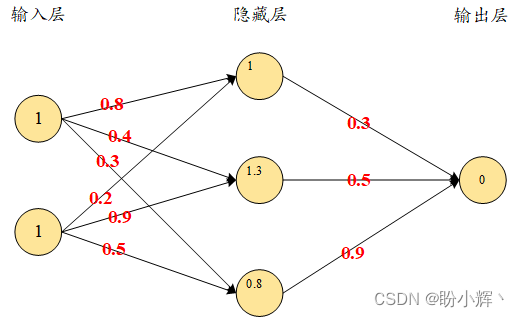
Next, we pass the hidden layer values through the nonlinear activation. Note that if we do not apply a nonlinear activation function to the hidden layers, the neural network will essentially be connected linearly from input to output, regardless of the number of hidden layers present.

3.2 Perform nonlinear activation

Activation functions help to model complex relationships between inputs and outputs, and using them allows for a high degree of nonlinearity. Some of the commonly used activation functions are as follows (wherex is input):
$$\begin{gathered} Sigmoid(x)=\frac{1}{1+e^{-x}} \\ ReLU(x)=\{\begin{array}{r}xx>0\\ 0x\le 0\end{array} \\ Tanh(x)=\frac{e^x-e^{-x}}{e^x+e^{-x}} \\ Linear(x)=x \end{gathered}$$
After applying the activation function, the activation visualization corresponding to the input values is as follows:

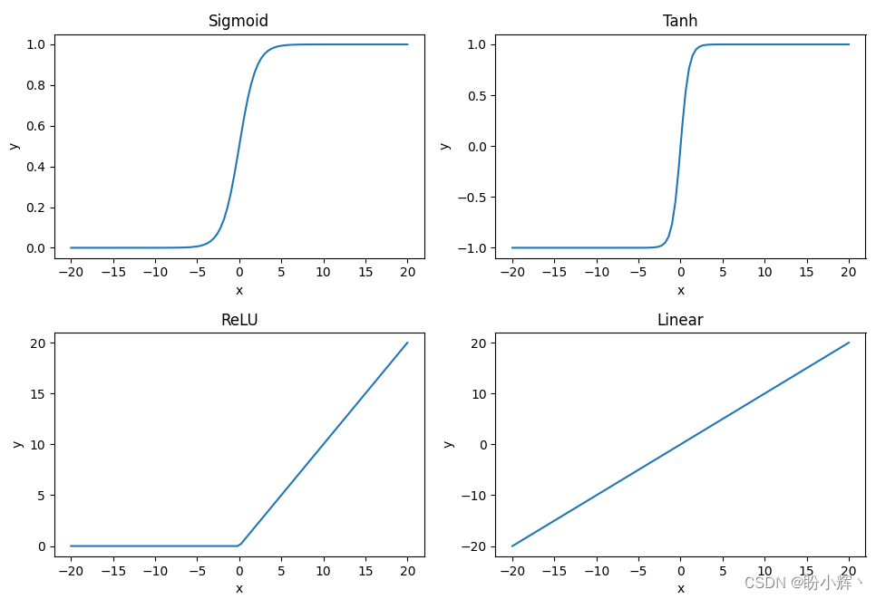
utilizationSigmoid activation function by applying to the hidden layersigmoid activation$S(x)$, the following results can be obtained:
$$\begin{gathered} a_{11}=sigmoid(1.0)=0.73 \\ {a}_{12}=sigmoid(1.3)=0.78 \\ {a}_{13}=sigmoid(0.8)=0.69 \end{gathered}$$

3.3 Calculating the output layer values

Next, we connect the hidden layer values after applying the activation function to the output layer by randomly initializing the weight values, and use the activated hidden layer values and weight values to compute the output values of the network:

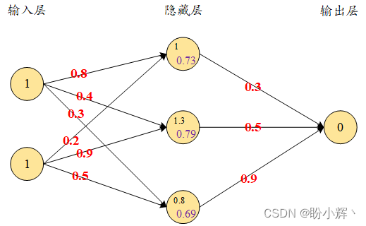
The sum of the products of the hidden layer values and the weight values is calculated to obtain the output values. In addition, to simplify the understanding of the details of how forward and backpropagation work, we temporarily ignore the bias terms in each cell (node):

$$output=0.73\times 0.3+0.79\times 0.5+0.69\times 0.9=1.235$$

Since we start with a set of random weights, the values of the output nodes have a large difference from the target value, and based on the above calculations we can see that the difference is1.235 (Our goal is to make the difference between the target value and the output value of the model0 ). In the next subsection, we will learn how to compute the loss value of the network in the current state.

3.4 Calculation of the value of the loss

Loss value (Loss values, also known as the cost functioncost functions ) is the value we need to optimize in the neural network. To understand how to calculate the loss value, we analyze the following two cases:

• Categorical (discrete) variable prediction
• Continuous variable forecasting

3.4.1 Calculating Losses in a Continuous Variable Prediction Process

Typically, when the variables are continuous, the average of the squares of the difference between the actual and predicted values can be calculated as the value of the loss, i.e., we try to minimize the mean square error by varying the values of the weights associated with the neural network:

$$\begin{gathered} J_{\theta }=\frac{1}{m}\sum _{i=1}^m(y_i-{\hat{y}}_i{)}^2 \\ {\hat{y}}_i={\eta }_{\theta }(x_i) \end{gathered}$$

Among them.$y_i$ is the actual output.${\hat{y}}_i$ It is made of neural networks$\eta$ (weighted$\theta$ ) The predicted output obtained by calculating the inputs of$x_i$，$m$ is the number of samples used for training in the dataset.
The key point is that for each different set of weights, the neural network will get a different loss value; ideally, we need to find the best set of weights that will make the loss zero, and in real scenarios, we need to find the set of weights that will make the loss value as close to zero as possible.
In the example in the previous subsection, assuming that the predictions are continuous values and the loss function uses the mean square error, the results are calculated as follows:

$$loss(error)=1.235^2=1.52$$

3.4.2 Computation of losses in the prediction process for categorical (discrete) variables

When the variable to be predicted is discrete (i.e., the variable has only a few categories), we usually use categorical cross-entropy (categorical cross-entropy) loss function. When the variable to be predicted has two different values, the loss function is binary cross-entropy (binary cross-entropy), the binary cross entropy is calculated as follows:

$$-\frac{1}{m}\sum _{i=1}^m(y_i(log(p_i)+(1-y_i)log(1-p_i))$$

The categorical cross entropy is calculated as follows:

$$-\frac{1}{m}\sum _{j=1}^C\sum _{i=1}^m{y}_{i}log(p_i)$$

Among them.$y$ is the true value corresponding to the output (i.e., the label of the data sample).$p$ is the predicted value of the output.$m$ is the total number of data samples.$C$ is the total number of categories.

An easy way to visualize cross-entropy loss is to look at the prediction matrix. Suppose we need to predict five categories in an image recognition problem – dog, cat, horse, sheep and cow. The neural network must contain five neurons in the last layer and use thesoftmax Activation function. At this point, the network will output the probability that a data sample belongs to each category. Assuming there are five images, the predicted probabilities are shown below, where the highlighted cell in each row corresponds to the true label of the image (also known as the target category, thetarget class)：

The sum of the probabilities in each row is1. In the first line, when the target isDog, the predicted probability is0.88 When the corresponding loss value is0.128; similarly, we can calculate other loss values, which are smaller when the probability of the correct category is higher. Since the probability lies between0 respond in singing1 Between, therefore, when the probability is1 When the minimum possible loss is0, and when the probability is0 When the maximum loss can be infinite, the final loss of the model is the average of the losses of all rows (training data samples).

3.5 Realization of forward propagation

The strategy to achieve forward propagation is as follows:

1. Neuron output values by multiplying input values by weights
2. Calculating the activation value
3. Repeat the first two steps on each neuron until the output layer
4. Compare the predicted output with the true value to calculate the loss value

We can encapsulate the above process into a function that takes the input data, the current neural network weights, and the true value as inputs to the function and returns the current loss value of the network:

import numpy as np
def feed_forward(inputs, outputs, weights):
    pre_hidden = np.dot(inputs, weights[0]) + weights[1]
    hidden = 1/(1+np.exp(-pre_hidden))
    pred_out = np.dot(hidden, weights[2]) + weights[3]
    mean_squared_error = np.mean(np.square(pred_out - outputs))
    return mean_squared_error

(1) Set the value of the input variable (inputs), weights (weights, randomly initialized if it is the first iteration) and the actual output of the data (outputs) asfeed_forward function’s arguments:

import numpy as np
def feed_forward(inputs, outputs, weights):

Since bias terms are added for each neuron node, the weight array contains not only the weights connecting the different nodes, but also the bias terms associated with the nodes in the hidden/output layer.

(2) By performing the input layer and weighting values (weights[0]) of the matrix multiplication (np.dot) to compute the hidden layer values, and the bias value (weights[1]) is added to the hidden layer, and the input layer can be connected to the hidden layer using the weights and bias values:

pre_hidden = np.dot(inputs, weights[0]) + weights[1]

(3) After obtaining the hidden layer values (pre_hidden) and abovesigmoid Activation function:

hidden = 1/(1+np.exp(-pre_hidden))

(4) This is accomplished by applying the hidden layer activation value (hidden) and weights (weights[2]that connects the hidden layer to the output layer) performs matrix multiplication (np.dot) computes the output layer values and then adds a bias term to the output (weights[3])：

pred_out = np.dot(hidden, weights[2]) + weights[3]

(5) Calculate the mean square error value for all data samples and return it:

mean_squared_error = np.mean(np.square(pred_out - outputs))
    return mean_squared_error

Among them.pred_out is the predicted output, whileoutputs is the actual output that the input should correspond to.

4. Reverse dissemination

4.1 Reverse propagation process

In forward propagation, we connect the input layer to the hidden layer and then connect the hidden layer to the output layer. At the first iteration, the weights are randomly initialized, and then the loss of the network at the current value of the weights is calculated. In backpropagation, we use the opposite approach. Using the loss values calculated from the forward propagation and updating the network weights with the goal of minimizing the loss values as much as possible, the network weights are updated in the following steps:

1. Make small changes to each weight in the neural network one at a time
2. Measurement weight changes ($\delta W$) at the time of the loss change ($\delta L$)
3. count$-k\frac{\delta L}{\delta W}$ Update the weights (where$k$ is the learning rate and is positive, an important hyperparameter in neural networks)

The update made to a particular weight is proportional to the reduction in the value of the loss, i.e., if changing a weight reduces the loss significantly, then the weight is updated more, but if changing the weight reduces the loss only slightly, then only a small update to the weight is required.
Execute on the entire datasetn times the above process (both forward and backward propagation), indicating that the model performs then classifier for individual things or people, general, catch-all classifierepoch The training (performed once is called aepoch)。
Since neural networks can often contain millions of weights, it is not optimal in practice to change the value of each weight and check the change in loss. The core idea of the above steps is to calculate the “loss variation” as the weights change, i.e., to calculate the gradient of the loss value with respect to the weights.
In this section, we will implement gradient descent from zero by updating one weight at a time a small amount at a time, but before we implement backpropagation, we first understand another key hyperparameter of neural networks: the learning rate (learning rate)。
Intuitively, the learning rate helps build more stable algorithms. For example, when determining the size of a weight update, we do not change it drastically all at once, but take a more cautious approach to update the weights slowly. This allows the model to achieve higher stability; in subsequent studies, we will also investigate how the learning rate helps improve network stability.

4.2 Gradient descent

The whole process of updating the weights to reduce the error value is called gradient descent (gradient descent). Stochastic gradient descent (stochastic gradient descent, SGD) is a method to minimize the error where random (stochastic) denotes randomly selecting a sample of training data from the dataset and making a decision based on that sample. Besides stochastic gradient descent, there are many other optimizers that can be used to reduce the loss values. We will also learn different optimizers in subsequent studies.
Next, we’ll learn how to use thePython Implementing backpropagation from scratch and describing how to backpropagate using the chain rule.

4.3 Implementing the Gradient Descent Algorithm

(1) Define the feedforward network and calculate the mean square error loss value:

from copy import deepcopy
import numpy as np
def feed_forward(inputs, outputs, weights):
    pre_hidden = np.dot(inputs, weights[0]) + weights[1]
    hidden = 1/(1+np.exp(-pre_hidden))
    pred_out = np.dot(hidden, weights[2]) + weights[3]
    mean_squared_error = np.mean(np.square(pred_out - outputs))
    return mean_squared_error

(2) Add a very small amount to each weight and bias term (0.0001), and a squared error loss value is computed for each weight and bias update.

establishupdate_weights function that updates the weights by performing gradient descent. The input to the function is the input to the networkinputsTargeted OutputsoutputsWeightingweights and the learning rate of the modellr：

def update_weights(inputs, outputs, weights, lr):

Since the weights need to be manipulated in a subsequent step, use thedeepcopy Make sure we can handle multiple copies of the weights without affecting the actual weights by creating three copies of the original set of weights passed as input to the function – theoriginal_weights、temp_weights respond in singingupdated_weights：

original_weights = deepcopy(weights)
    temp_weights = deepcopy(weights)
    updated_weights = deepcopy(weights)

commander-in-chief (military)inputs、outputs respond in singingoriginal_weights pass on tofeed_forward function that uses the original set of weights to compute the loss value (original_loss)：

original_loss = feed_forward(inputs, outputs, original_weights)

Traverse all layers of the network:

for i, layer in enumerate(original_weights):

The example neural network contains four parameter lists, the first two lists represent the weight and bias term parameters that connect the input to the hidden layer, and the other two represent the weight and bias parameters that connect the hidden layer to the output layer. The loop iterates over all the parameters, since each parameter list has a different shape, using thenp.ndenumerate Loop through each parameter in the given list:

for index, weight in np.ndenumerate(layer):

Store the original set of weights in thetemp_weights, loop through each parameter and add a smaller value to it, and compute the new loss using the new set of weights from the neural network:

temp_weights = deepcopy(weights)
            temp_weights[i][index] += 0.0001
            _loss_plus = feed_forward(inputs, outputs, temp_weights)

In the above code, thetemp_weights reset to the original set of weights, since in each iteration a parameter needs to be updated in order to compute the loss when a small update is made to the parameter.

Calculate the gradient (change in loss value) due to the change in weights:

grad = (_loss_plus - original_loss)/(0.0001)

This process of updating the parameters by a very small amount and then computing the gradient is equivalent to the process of differentiation.

Updating weights by loss changes and using the learning ratelr Make weight changes more stable:

updated_weights[i][index] -= grad*lr

After all parameter values have been updated, return the updated weight values –updated_weights：

return updated_weights, original_loss

Another hyperparameter to consider in neural networks is the batch size in calculating loss values (batch size). In the above example, we used all data points to calculate the loss values. However, in practice, datasets typically contain tens of thousands or even millions of data points, and the incremental contribution of too many data points in calculating the loss value follows a law of diminishing returns, with a much smaller batch size compared to the total number of samples in our data. When training the model, a batch of data points is used one at a time to apply gradient descent to update the network parameters until we are at the end of a training cycle (epoch) within traversing all data points. When building a model, the batch size is usually between32 until (a time)1024 Between.

4.4 Implementing Backpropagation Using Chaining Laws

We have learned how to compute the loss gradient with respect to the weights by making a small update to the weights and then computing the difference in loss before and after the weight update. When the network parameters are large, updating the weight values in this way requires a large number of computations to obtain the loss values, and therefore requires larger resources and time. In this section, we will learn how to utilize the chain rule to obtain the loss gradient with respect to the weight values.
In the example in the previous subsection, the first iteration outputs a prediction of1.235. The weights and hidden layer values and hidden layer activation values are denoted respectively as$w$、$h$ respond in singing$a$：

In this section, we will learn how to use the chain rule to compute the loss value with respect to the$w_{11}$ of the gradient, other weights and bias values can be computed using the same approach. In addition, to make it easier to understand the chain rule, we only need to deal with one data point, where the inputs are{1,1}The output target value is{0}。
To calculate the value of the loss with respect to$w_{11}$ of the gradient, one can get an idea of all the intermediate components to be included in the calculation of the gradient by using the following diagram (labeled with black markers – the$h_{11}$、$a_{11}$ respond in singing$\hat{y}$)：

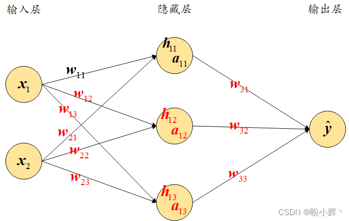
The loss value of the network is expressed as follows:

$$Los{s}_{MSE}(C)=(y-\hat{y}{)}^2$$

Predicted output value$\hat{y}$ The calculations are as follows:

$$\hat{y}=a_{11}\ast w_{21}+a_{12}\ast w_{22}+a_{13}\ast w_{23}$$

The hidden layer activation value (sigmoid activation) is calculated as follows:

$$a_{11}=\frac{1}{1+e^{-h_{11}}}$$

The hidden layer values are calculated as follows:

$$h_{11}=x_1\ast w_{11}+x_2\ast w_{21}$$

Calculation of the value of the loss$C$ The change in the weights relative to the$w_{11}$ The change:

$$\frac{\partial C}{\partial w_{11}}=\frac{\partial C}{\partial \hat{y}}\ast \frac{\partial \hat{y}}{\partial a_{11}}\ast \frac{\partial a_{11}}{\partial h_{11}}\ast \frac{\partial h_{11}}{\partial w_{11}}$$

The above equation is called the chain rule (chain rule), in the above equation we build a chain of partial differential equations to perform partial differentiation for each of the four components and finally calculate the derivative values of the loss values with respect to the weights$w_{11}$. The individual partial derivatives in the above equation are calculated as follows.

Loss value relative to predicted output value$\hat{y}$ The partial derivatives of are as follows:

$$\frac{\partial C}{\partial \hat{y}}=\frac{\partial }{\partial \hat{y}}(y-\hat{y}{)}^2=-2\ast (y-\hat{y})$$

Predicted output value$\hat{y}$ Activation value relative to the hidden layer$a_{11}$ The partial derivatives of are as follows:

$$\frac{\partial \hat{y}}{\partial a_{11}}=\frac{\partial }{\partial a_{11}}(a_{11}\ast w_{21}+a_{12}\ast w_{22}+a_{13}\ast w_{23})=w_{21}$$

Hidden layer activation value$a_{11}$ Relative to the hidden layer value$h_{11}$ The partial derivatives are as follows:

$$\frac{\partial a_{11}}{\partial h_{11}}=a_{11}\ast (1-a_{11})$$

Hidden Layer Value$h_{11}$ Relative to the weight value$w_{11}$ The partial derivatives are as follows:

$$\frac{\partial h_{11}}{\partial w_{11}}=\frac{\partial }{\partial w_{11}}(x_1\ast w_{11}+x_2\ast w_{21})=x_1$$

Therefore, the value of the loss relative to the$w_{11}$ The gradient of can be expressed as:

$$\frac{\partial C}{\partial w_{11}}=-2\ast (y-\hat{y})\ast w_{21}\ast a_{11}\ast (1-a_{11})\ast x_1$$

As you can see from the above equation, we are now able to directly calculate the effect of small changes in the weight values on the loss values (the gradient of the loss relative to the weights) without having to recalculate the forward propagation. Next, the weight values are updated:

$$updated\_weight=original\_weight-lr\ast gradient\_of\_loss$$

5. Combining forward and backward propagation

In this section, we will construct a simple neural network with hidden layers (connecting inputs and outputs), using the simple dataset presented in the previous subsection and utilizing theupdate_weights function performs backpropagation to obtain optimal weights and bias values. The model is defined as follows:

1. The input is connected to a hidden layer with three neurons (nodes).
2. The hidden layer is connected to an output layer with one neuron

Next, use thePython Creating Neural Networks:

(1) Import relevant libraries and define datasets:

import numpy as np 
from copy import deepcopy
import matplotlib.pyplot as plt
x = np.array([[1,1]])
y = np.array([[0]])

(2) Randomly initialize the weights and bias values.

There are three neurons in the hidden layer, and each input node is connected to a hidden layer neuron. Thus, there are six weight values and three bias values, with each hidden layer neuron containing one bias and two weights (each input connection to a hidden layer neuron corresponds to one weight); the final layer has one neuron connected to the three units of the hidden layer, and thus contains three weights and one bias value. The randomly initialized weights are as follows:

W = [
    np.array([[-0.0053, 0.3793],
              [-0.5820, -0.5204],
              [-0.2723, 0.1896]], dtype=np.float32).T, 
    np.array([-0.0140, 0.5607, -0.0628], dtype=np.float32), 
    np.array([[ 0.1528, -0.1745, -0.1135]], dtype=np.float32).T, 
    np.array([-0.5516], dtype=np.float32)
]

where the first parameter array corresponds to the input layer that connects the input layer to the hidden layer of the2 x 3 weight matrix; the second parameter array represents the bias value associated with each neuron of the hidden layer; the third parameter array corresponds to the output layer that connects the hidden layer to the3 x 1 weight matrix, and the last parameter array represents the bias values associated with the output layer.

(3) exist100 classifier for individual things or people, general, catch-all classifierepoch Performs forward and backward propagation within, using thefeed_forward respond in singingupdate_weights function.

During training, the weights are updated and the loss values and updated weight values are obtained:

def feed_forward(inputs, outputs, weights):     
    pre_hidden = np.dot(inputs,weights[0])+ weights[1]
    hidden = 1/(1+np.exp(-pre_hidden))
    out = np.dot(hidden, weights[2]) + weights[3]
    mean_squared_error = np.mean(np.square(out - outputs))
    return mean_squared_error

def update_weights(inputs, outputs, weights, lr):
    original_weights = deepcopy(weights)
    temp_weights = deepcopy(weights)
    updated_weights = deepcopy(weights)
    original_loss = feed_forward(inputs, outputs, original_weights)
    for i, layer in enumerate(original_weights):
        for index, weight in np.ndenumerate(layer):
            temp_weights = deepcopy(weights)
            temp_weights[i][index] += 0.0001
            _loss_plus = feed_forward(inputs, outputs, temp_weights)
            grad = (_loss_plus - original_loss)/(0.0001)
            updated_weights[i][index] -= grad*lr
    return updated_weights, original_loss

(4) Plotting loss values:

losses = []
for epoch in range(100):
    W, loss = update_weights(x,y,W,0.01)
    losses.append(loss)
plt.plot(losses)
plt.title('Loss over increasing number of epochs')
plt.xlabel('Epochs')
plt.ylabel('Loss value')
plt.show()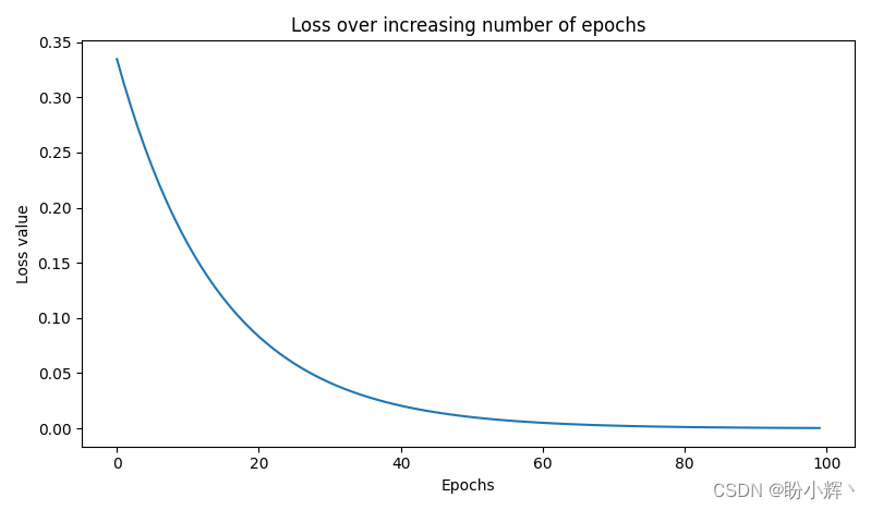

The value of the loss was initially0.33 around the same time, and then gradually declining to0.0001 around, which indicates that the weights are adjusted according to the input-output data, and we can get the desired target value by adjusting the network parameters when given the inputs. The adjusted weights are as follows:

print(W)
'''Output results
[array([[ 0.01424004, -0.5907864 , -0.27549535],
       [ 0.39883757, -0.52918637,  0.18640439]], dtype=float32), array([ 0.00554004,  0.5519136 , -0.06599568], dtype=float32), array([[ 0.3475135 ],
       [-0.05529078],
       [ 0.03760847]], dtype=float32), array([-0.22443289], dtype=float32)]
'''

utilizationNumPy Arrays are not the best way to build a network from scratch, but they can provide a solid foundation for understanding how neural networks work.

(5) After obtaining the updated weights, the inputs are predicted and the output values are calculated by passing the inputs to the network:

pre_hidden = np.dot(x,W[0]) + W[1]
hidden = 1/(1+np.exp(-pre_hidden))
pred_out = np.dot(hidden, W[2]) + W[3]
print(pred_out)
# [[-0.0174781]]

outputs-0.017This value is very close to the expected output0, by training moreepoch，pred_out The value will be closer to0。

6. Summary of the neural network training process

Training the neural network is mainly done by repeating two key steps, i.e., forward propagation and back propagation at a given learning rate, and ultimately the neural network architecture gets the best weights.
In forward propagation, we apply a set of weights to the input data, pass them to the defined hidden layer, perform a nonlinear activation on the output of the hidden layer, and then connect the hidden layer to the output layer by multiplying the hidden layer node values with another set of weights to estimate the output values; ultimately, we compute the loss that corresponds to a given set of weights. Note that the values of the weights are randomly initialized for the first forward propagation.
In backpropagation, the loss value (error) is reduced by adjusting the weights in the direction where the loss decreases, and the weights are updated by a magnitude equal to the gradient multiplied by the learning rate.
The process of forward and backward propagation is repeated until the smallest possible loss is obtained, and at the end of training the neural network has weighted its$\theta$ Adjust the tuning to near-optimal values in order to obtain the desired output.

wrap-up

In this section, we learned about the differences between traditional machine learning and artificial neural networks and how to connect the layers of the network before implementing forward propagation to compute the loss value corresponding to the current weights of the network; backpropagation was implemented to optimize the weights to achieve the goal of minimizing the loss value. And implemented all the key components of the network – forward propagation, activation function, loss function, chain rule, and gradient descent – to build and train a simple neural network from scratch.

Series Links

PyTorch Deep Learning in Action (2) – PyTorch Basics
PyTorch Deep Learning in Action (3) – Building Neural Networks with PyTorch
PyTorch deep learning in practice (4) – common activation function and loss function details
PyTorch Deep Learning in Action (5) – Computer Vision Basics
PyTorch Deep Learning in Action (6) – Neural Network Performance Optimization Techniques
PyTorch Deep Learning in Action (7) – Impact of Batch Size on Neural Network Training
PyTorch Deep Learning in Action (8) – Batch Normalization